−
a y −
a y
i
i
i
i
...
1
1
2
2
dA i− dA
128
New Approaches in Automation and Robotics
4. In the following steps 4-7 identification procedures described in details in section 3 are
realized.
5. The first, the second, the third and the fourth moments of the residuum ηi are
estimated.
6. Identifiability criterion for EB(k,l) process is checked for the series of residuum. If fitting
elementary bilinear model is possible, one can continue in the step 7. If not, one should
move to the step 12.
7. The structure (k,l) of the EB(k,l) model is established on the base of the third moment for
residuum.
8. The values of β and (2)
m are calculated using e.g. one of the moments’ methods.
kl
w
9. For the assumed prediction horizon h and the estimated polynomial A(D) the
diophantine equation (58) is solved, and the parameters f , k=1,…,h-1 of the
k
polynomial F(D) as well as the parameters g , j=1,…,dA-1 of the polynomial G(D) are j
calculated. Then, if the prediction horizon h ≤ min( k, l) , prediction algorithm is
designed either on the base of the Theorem 1 -- for the EB(k,l) model of the residuum, or
on the base of the Theorem 2 -- for the EB(k,k) model of the residuum.
10. The designed prediction algorithm is tested on the testing set. STOP.
11. If h > min( k, l) then move to the step 12.
12. Design linear prediction algorithm e.g. [1], [4]: ˆ y
=
+
(
G D) y
i
|
h i
i
13. Test it on the training set. STOP.
The above prediction strategy was tested for simulated and real world time series. In the
next section, the strategy is applied to series of sunspot numbers and MVB prediction is
compared with the non-linear prediction performed using the benchmark SETAR model,
proposed by Tong (Tong, 1993).
4.4 Sunspot number prediction
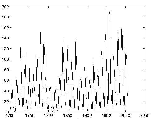
Sunspots events have been observed and analysed for more than 2000 years.
Sunspot
number
year
Fig. 4. Sunspot events

Bilinear Time Series in Signal Analysis
129
The earliest recorded date of a sunspot event was 10 May 28 BC. The solar cycle was first
noted in 1843 by the German pharmaceutical chemist and astronomer, Samuel Heinrich
Schwabe as a result of 17 years of daily observations. The nature of solar cycle, presented in
the Fig. 4 characterized by a number of sunspots that periodically occurs, remains a
mystery to date. Consequently, the only feasible method to predict future sunspot number is
time series modeling and time series prediction. Linear prediction do not give acceptable
results hence, the efforts are made to improve the prediction using nonlinear models and
nonlinear methods. Tong (Tong, 1993) has fitted a threshold autoregressive (SETAR) model
to the sunspot numbers of the period 1700-1979:
1.92
⎧⎪
+ 0.84 Y +
−
+
−
−
Y−
Y−
Y−
Y
i
0.07 i
0.32 i
0.15 i
0.20
1
2
3
4
i−5
⎪⎪⎪
1
−
⎪ 0.00 Y +
−
+
+
+
≤
−
Y−
Y−
Y−
Y−
e
when Y
⎪
i
0.19 i
0.27 i
0.21 i
0.01 i
i
i−
11.93
6
7
8
9
10
8
Y = ⎪
(62)
i
⎨⎪⎪⎪⎪
2
⎪4.27 + 1.44 Y −
−
+
> 11.93
⎪⎩
−
Y−
Y−
e
when Y
i
0.84 i
0.06 i
i
1
2
3
i−8
The real data were transformed in the following way:
Y =
+ y − (63)
i
2( 1
i
1)
where y is the sunspot number in the year 1699+i.
i
Based on the model (62) prediction for the period 1980-2005 was derived, and used as a
benchmark for comparison with the prediction, performed in the way discussed in the
paper. The HLB model (64) was then fitted to the sunspot numbers, coming from the same
period 1700-1979, under the assumption that the linear part of the HLB model satisfies the
coincidence condition.
Y =
Y +
+
−
Y
η
i
0.81 i
0.21
1
i−8
i (64)
η = e +
η − e
i
i
0.02 i 7 i−7
The Y is a variable transformed in the same way as in the Tong’s model (62), and the
i
variance of residuum is var( η) = 8.13 .
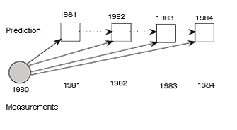
1981
1982
1983
1984
prediction
1980
1981
1982
1983
1984
real data
Fig. 5. Scheme of prediction calculation
Sunspot events prediction for the period 1981—2005 was performed according to the
scheme showed in the Fig. 5. One step ahead prediction ˆ y
calculated at time i depends on
i+1| i
the previous data and the previous predictions. Prediction algorithm has the form specified
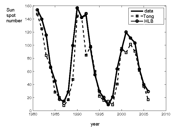
in Theorem 2.For the data transformed according to (63) predictions obtained based on
Tong’s model and the HLB model are compared in the Fig. 6.
130
New Approaches in Automation and Robotics
Fig. 6. Prediction for the period 1981-2005 based on Tong’s and HLB models
The HLB prediction is evidently more precise than the one derived on the base of the Tong’s
model. Sum of squares of the Tong’s prediction errors was:
4
S =
×
,
T
1.07 10
while sum of squares of the HLB prediction errors was:
3
S
=
×
MLB
1.70 10
Data transformation (63) is not natural for minimum variance prediction. Therefore, HLB
model was once more identified, for the data transformed in the following way:
y − y
i
Y =
. (65)
i
var( y)
This time the following HLB model was identified:
Y =
Y −
+
+
−
Y−
Y
η
i
0.80 i
0.29 i
0.52
1
7
i−8
i (66)
η = e +
η − e
i
i
0.08 i 3 i−3
and variance of the residuum var( η) = 0.24. Prediction algorithm was built on the base of
model (66) in a way specified in Theorem 2. The sum of squares of the HLB prediction
errors was this time:
S
=
,
MLB
30
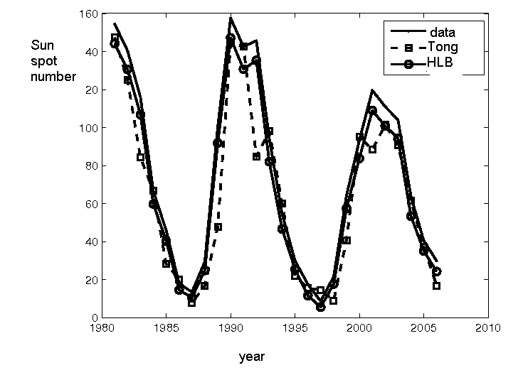
hence, higher quality of the HLB prediction was obtained this time than previously. Fig. 7
illustrates prediction for the period 1981-2005, obtained on the base of Tong’s model (62),
built on the data transformed according to (63), and on the base of HLB model (66).
Tong (Tong, 1993) after discussion with Sir David Cox, one of the greatest statisticians in XX
century, defined genuine prediction, as the prediction of data that are entirely not known at
the stage of prediction establishing. The idea is illustrated in the following scheme, and is
known also as a multi-step prediction.
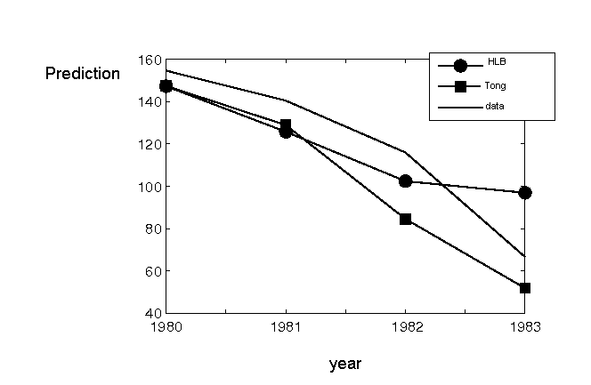
In 1979, genuine prediction of sun spot numbers was established for years 1980—1983 on
the base of Tong, and HLB models. Sums of squares of the prediction errors were equal to
347 and 342, respectively. The results are showed in the Fig. 9.
Bilinear Time Series in Signal Analysis
131
Fig. 7. Prediction for the period 1981-2005 based on Tong’s and HLB models.
Fig. 8. Illustration of genuine prediction
Fig. 9. Genuine prediction for the period 1980-84
5. Resume
In the chapter, a new method of time series analysis, by means of elementary bilinear time
series models was proposed. To this aim a new, hybrid linear – elementary bilinear model
132
New Approaches in Automation and Robotics
structure was suggested. The main virtue of the model is that it can be easily identified.
Identification should be performed for the linear and the non-linear part of the model
separately. Non-linear part of the model is applied for residuum, and has elementary
bilinear structure. Model parameters may be estimated using one of the moments’ methods,
because relations between moments and parameters of elementary bilinear time series
models are known.
Based on HLB model, minimum-variance bilinear prediction algorithm was proposed, and
the prediction strategy was defined. The proposed prediction strategy was than applied to
one of the best-known benchmark – sunspot number prediction. Prediction efficiency
obtained with the use of HLB model, and bilinear prediction algorithm, in the way described
in the paper, occurred much better than the efficiency obtained on the base of SETAR model,
proposed by Tong.
6. References
Bond, S.; Bowsher, C. &, Windmeijer F. (2001). Criterion-based inference for GMM in
autoregressive panel data models, Economic Letters, Vol.73
Brunner, A. & Hess, G. (1995). Potential problems in estimating bilinear time-series models.
Journal of Economic Dynamics & Control, Vol. 19, Elsevier
Dai, H. & Sinha, N. (1989). Robust recursive least squares method with modified weights for
bilinear system identification. IEE Proceedings, Vol. 136, No. 3
Faff R. & Gray P. (2006). On the estimation and comparison of short-rate models using the
generalised method of moments. Journal of Banking & Finance, Vol. 30
Granger, C. & Andersen A., (1978). Nonlinear time series modeling, In: Applied Time series
analysis, Academic Press.
Granger, C. & Terasvirta, T. (1993). Modelling nonlinear Economic Relationships, “ Oxford
University Press, Oxford
Gourieroux, C.; Monfort A. & Renault E. (1996). Two-stage generalized moment method
with applications to regressions with heteroscedasticity of unknown form, Journal
of Statistical Planning and Interference, Vol.50
Kramer, M. & Rosenblatt, M. (1993). The Gaussian log likehood and stationary sequences,
In: Developments in time series analysis, Suba Rao, T. (Ed.), Chapman & Hall
Martins, C. (1997). A note on the autocorrelations related to a bilinear model with non-
independent shocks. Statistics & Probability Letters, Vol. 36
Martins, C. (1999). A note on the third order moment structure of a bilinear model with non
independent shocks. Portugaliae Mathematica, Vol.56
Mohler, R. (1991). Nonlinear systems. Vol.II. Applications to bilinear control. Prentice Hal
Nise, S. (2000). Control systems engineering. John Wiley & Sons
Priestley, M. (1980). Spectral analysis and time series. Academic Press
Schetzen, M. (1980). The Volterra & Wiener Theories of Nonlinear Systems. Wiley-Interscience,
New York
Subba Rao, T. (1981). On the theory of bilinear models. Journal of Royal Statistic Soc iety,
Vol.B, 43
Tang, Z. & Mohler, R. (1988). Bilinear time series: Theory and application. Lecture notes in
control and information sciences, Vol.106
Therrien, C. (1992). Discrete random signals and statistical signal processing, Prentice Hall
Tong, H. (1993). Non-linear time series. Clarendon Press, Oxford
Wu Berlin, (1995). Model-free forecasting for nonlinear time series (with application to
exchange rates. Computational Statistics & Data Analysis. Vol. 19
Yaffee, R. (2000). Introduction to time series analysis and forecasting, Academic Press
8
Nonparametric Identification of
Nonlinear Dynamics of Systems
Based on the Active Experiment
Magdalena Boćkowska and Adam Żuchowski
Szczecin University of Technology
Poland
1. Introduction
Identification is a process (measured experiment and numerical procedure) aiming at
determining a quantitative model of the examined object’s behaviour. Identification of
dynamics is a process which tries to define a quantitative model of variation of system state
with time. The goal in the experiment is to measure inputs and outputs of the examined
object, the system excitations and reactions. In special cases the model can be treated as a
“black box” but it always has to be connected with physical laws and can not be inconsistent
with them.
The most commonly used models of system dynamics are differential equations – general
nonlinear, partial, often nonlinear ordinary, rarely linear ordinary, additionally non-
stationary and with deviated arguments. Sometimes one considers discrete-time models
presented in a form of difference equations, which are simplified models of a certain kind.
Integral equations, functional equations etc. are models of a different kind.
If a model structure is a priori known or if it can be assumed, the identification consists in
determination of model parameters and it is defined as parametric identification. If the full
model structure or its part is not known, nonparametric identification has to be used.
In domain of linear models an equivalence of linear ordinary differential equations is
transfer function, transient response or frequency response. They can be obtained using
experiments of various types: passive – observation of inputs or outputs without interaction
upon object or active – excitation of the examined object by special signals (determined:
impulse, leap, periodic, a periodic, lottery: white noise, coloured noise, noise with
determined spectrum…).
Many possibilities lead to a variety of identification methods. In the last decades various
identification methods have been developed. Rich bibliography connected with this
thematic includes Uhl’s work (Uhl, 1997) which describes computer methods of
identification of linear and nonlinear system dynamics, in time domain and also frequency,
with short characteristic and a range of their applications.
There are many methods of parametric and nonparametric identifications of linear
dynamics of systems (Eykhoff, 1980), (Iserman, 1982), (Söderström & Stoica, 1989). There are
fewer useful methods applied for systems with nonlinear dynamics (Billings & Tsang, 1992),
(Greblicki & Pawlak, 1994), (Haber & Keviczky, 1999), thereby a presented simple solution
134
New Approaches in Automation and Robotics
can be very useful in identification of the structure of a model of nonlinear dynamics of 1st
and higher orders.
The method of identification has to be adapted to planned and possible experiments and the
type of the assumed model structure. Active identification is more precise than that which is
based on a passive experiment. A parametric identification connects optimisation with the
regression method which allows to decrease the influence of disturbances and consequently
increases accuracy of the model parameters. The precision of identification depends on the
degree of disturbances elimination, errors of measured methods and accuracy of measuring
devices.
The input and output are often measured as disturbed signals. The parametric identification
for non-linear systems based on the method of the averaged differentiation with correction
was introduced in the paper (Boćkowska, 2003). The method of averaged differentiation
allows to filter distorted signals and to obtain their derivatives. Thanks to the correction
procedure one can obtain such values of the corrected averaged signals and their
derivatives, which are very close to their real values.
2. Averaged differentiation method with correction as regularization filter
The method of averaged differentiation is a regularization filter which allows to determine
useful signals and their derivatives based on the disturbed signals available from
measurement. Operation of averaged differentiation can be used to evaluate a derivative of
any function of signal and time, and averaged signals can be used in estimation of model
parameters. Nevertheless its application is not sufficient to determine nonlinearity such as
multiplication or other non-linear functions of derivatives with different order. The problem
can be solved through connecting the operation with specially designed procedures of
correction. Hence one can obtain such values of the corrected averaged signals and their
derivatives, which are very close to their real values and so can be used to determine
nonlinearity with different structures, good enough to estimate parameters of nonlinear
models.
2.1 Definition of averaged differentiation method
If the signal x(t) is passing through the window g(v) with the width ±d starting from the
moment t0, Fig. 1, then the output of the window is the signal (Kordylewski & Wach, 1988):
d
(
x t ) =
0 g
∫ (xt + v)⋅
0
g(v dv
)
.
(1)
−d
If the function x(t) is differentiable, then it x(t0+v) can be expanded into Taylor series in the
neighbourhood of the point t0:
∞
i
v
(
x t + v) =
0
∑ ⋅ (i)
x (t0 ) . (2)
i=0 !
i
Denoting the moments of the measurement window as:
d
m =
i
∫ iv ⋅g(v dv
)
(3)
−d
Nonparametric Identification of Nonlinear Dynamics of Systems Based on the Active Experiment 135
the window response takes the form:
∞ m
(