⎝ ⎠ ⎥
1⎣
⎦
and corresponding plots for r=1÷6 are shown in Figure 7.
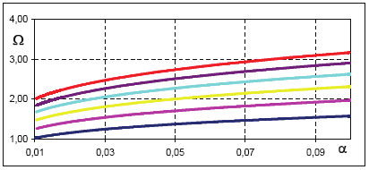
Figure 8 presents variability of Ωα versus α in the range 0.01 ≤ α ≤ 0.1. The relationship
Ωα=f(α) in an analytical form is needed to calculate quickly the optimal width of the
measurement window d for a given output and its pass band frequency fp according to (51).
The approximation of this relation can be evaluated using (51) and (47). The courses in the
given range were approximated by an exponential function:
P
Ωα apr
= S ⋅ α
(53)
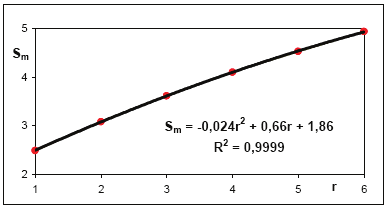
with very good fitting using the regression method. The results: the values of the coefficients
S and P as well as correlation coefficients R are shown in Table 2. The mean value of the
exponent Pm is equal to 0.197 and was accepted as constant. The new values of coefficients
Sm for Pm are also presented in Table 2. For Sm and r the quadratic dependence was found as
it is shown in Figure 9.
Fig. 7. The spectrum of the corrected Nuttall window of 1st to 6th order versus Ω.
146
New Approaches in Automation and Robotics
Fig. 8. The normalised frequency Ω versus the accuracy α of transmission of the useful
signal.
r
1 2 3 4 5 6
S 4.9755 4.5838 4.1065 3.6324 3.0745 2.4184
P 0.1991 0.2006 0.1971 0.1982 0.1961 0.1882
R 0.9997 0.9997 0.9996 0.9997 0.9998 0.9995
Sm 4.941 4.529 4.105 3.618 3.083 2.49
Table 2. Parameters of the approximate exponential function to the order r of the
measurement window.
Fig. 9. Variability of Sm versus r.
The result approximate relation, who determines the variability of Ωα versus r, is as follows:
2
197
.
0
Ωα apr
= (− 024
.
0
⋅ r + 66
.
0
⋅ r + .
1 86) ⋅ α
(54)
The correlation coefficients between the data, which was obtained on the basis of the
corrected window spectrum and the other calculated on the basis of the above mentioned
Nonparametric Identification of Nonlinear Dynamics of Systems Based on the Active Experiment 147
Equation (53), are still close to unity. The needed width of the measurement window can be
expressed in seconds, using (54) and measurement step relating to:
( 0
− .024 ⋅ r2 + 0 66
. ⋅ r + 1 86
. )
197
.
0
⋅ α
dopt =
.
(55)
(4 ⋅ f ⋅ step)
p
3. Identification of non-linear system dynamics
3.1 Parametric identification
The proposed procedure, the averaged differentiation operation with correction, can be
applied to evaluation of the parameters of the model of the system dynamics if the model
structure is known and corresponds in general to the differential equations of the kind:
y(n)(t) = F(y,y(1) ,
...
, y(n−1),x,x(1)
,
...
, x(n),A0 ...
, ,B0 ,
...
, D)
(56)
which can be written down as the following equation:
n
n−1
y(n)(t) = ∑A F
−
−
j ⋅ jx (y,Ky(n 1) , x,Kx(n) )⋅ x( j) − ∑B ⋅ F
j
jy (y,Ky(n 1) , x,Kx(n) )⋅ y( j) + D (57)
j=0
j=0
Taking into account all the measured data samples N, to which the model with the
parameters Aj, Bj and D must be fitted we can present the system in the matrix form:
⎡ A0 ⎤
⎢ ... ⎥
⎡y(n)⎤
⎢
⎥
1
⎢
⎥
⎢ A ⎥
(n)
n
⎢
⎥
⎢
⎥
y
Yn = XY ⋅ PAR
Yn
where
,
2
=
PAR
,
=
⎢
⎥
⎢ B0 ⎥
,
...
⎢
⎥
⎢ ... ⎥
⎢y(n)⎥
⎢
⎥
⎣ N ⎦
⎢Bn−1⎥
⎢ D ⎥
⎣
⎦
⎡ F
−
⎤
⋅
⋅
⋅
⋅
0x,1 x1
... Fnx,1 x(n) F0y,1 y1 ... Fny,1 y(n 1) 1
1
1
⎢
⎥
⎢ F
⋅ x
... F
⋅ x(n) F
⋅ y
... F
⋅ y(n−1) 1⎥
XY
0x,2
2
nx,2
2
=
0y,2
2
ny,2
2
⎢
⎥
(58)
...
...
...
...
...
...
...
⎢
⎥
⎢F
⋅ x
... F
⋅ x(n) F
⋅ y
... F
⋅ y(n−1) 1⎥
⎣ 0x,N N
nx,N
N
0y,N
N
ny,N
N
⎦
The system (58) with respect to some or all parameters Aj, Bj and D can be non-linear or
quite linear. In case of nonlinearity, non-linear optimisation has to be applied, for instance
by the simplex search method. An initial estimation of the parameters can be carried out
either by omitting nonlinearities, if this is possible, or by using another estimation
procedure. It is advisable to try several sets of starting values to make sure that the solution
gives relatively consistent results. The obtained result for a given optimal averaging width
dopt of the measurement window g(v) does not have to be an optimum. The verification of
the result of the identification, the model parameters, can be done through the
148
New Approaches in Automation and Robotics
determination of the mean square deviation between the output signal y and the model
response obtained through the simulation ys for the assigned parameters:
N
2
2
J = ∑(ys − y) = ys − y .
(59)
i=1
Both signals y and ys must be averaged and corrected. The minimum of criteria J proves the
result of non-linear optimisation and correctness of the choice of dopt.
3.2 Nonparametric identification of nonlinear dynamics of 1st order of systems based
on the active experiment (Boćkowska & Żuchowski, 2007)
Despite the fact that the presented method is nonparametric, its usefulness is limited to
systems dynamics with structure described by the following differential equation:
y(1) ⋅ (
ϕ x,y) + y ⋅ f(x,y) = x .
(60)
Thanks to the fact that the measured window is an even function, the method of the
averaged differentiation does not introduce any time shift between signals: the signals
measured for example y(1)(t0) and those who were averaged y(1)(t0)g. The corrected signals
are not shifted in relation to the measured signals, because the correction procedure is also
even.
An active experiment ensures that a rich spectrum signal is fed into the system input. A rich
spectrum can be achieved when a periodic signal with a modulated amplitude and
frequency is applied, for example:
(
x t) = A(t) ⋅ sin(t ⋅ (
ω t) + φ0) .
(61)
Averaged and corrected courses of signals x(t), y(t) and y(1)(t) should be obtained and the
plots of these courses created. The time moments for which y(1)(t)=0 can be easily obtained
and correspond to the points of the static characteristics of the examined object:
y ⋅ f(x,y) = x .
(62)
Next, the values of the second unknown function ϕ(t) can be defined using all the values of
both averaged and corrected signals.
The goal of the presented method is not the determination of the static characteristic, but
that of the function f(x,y). These two can produce the same or similar graphs, but they are
not always the same mathematically. It means that the structure of the function f(x,y) can
not be concluded from the relation y(x) without additional assumptions. The functions f and
ϕ can be the functions only of x or y or of both signals together. Hence, various models can
be created and some of them differ from the true model. The regression method should be
used in order to determine the functions f and ϕ on the basis of the plots of the following
relations:
x
x − y ⋅ f(x,y)
f(x,y) = z1 =
,
(
ϕ x,y) = z2 =
(63)
(1)
y
y
in the co-ordinate system x, y, z1 and x, y, z2. An input with a rich spectrum enables to
obtain a big collection of different points x, y, z1, z2.
Nonparametric Identification of Nonlinear Dynamics of Systems Based on the Active Experiment 149
The examined object can have the dynamics of an order higher than one. In this case the
obtained static characteristic is different from the real one and the change of the form of the
signal x(t) leads to other results. Hence, it is a good control test of the correctness of the
dynamics order.
The identified model should be obviously verified using numerical simulation.
A comparison between simulation results and measured data should also be carried out.
3.3 Nonparametric identification of nonlinear dynamics of 2nd order of systems
The consideration relates to the models of system dynamics with the following structure:
y(2) ⋅F2 (x,y,y(1))+ y(1) ⋅F1(x,y,y(1))+ F0 (x,y,y(1))= x .
(64)
The averaged corrected values of signals x, y, y(1) and y(2) are used. At first the relation
corresponding to static characteristics should be determined – a steady state, when y(1)(t)=0,
y(2)(t)=0 and x(t)=x=const.:
F0(x,y 0
, ) = x .
(65)
Usually the function F0(x,y) is independent at y(1)(t), hence the substitute relation can be
obtained:
y = (
φ x) .
(66)
Next, the values of x, y corresponding to the extreme values of the first derivative should be
chosen, for which:
y(2)(t) = 0.
(67)
The knowledge of the function F0(x,y), which was determined in the first step and multiple
chosen values of y(1)ex in the second step allow us to evaluate the structure of the function
F1(x,y,y(1)):
x − F x, y
1
F (
(1)
x, y,y )
0 (
)
=
.
(68)
(1)
y ex
In a particular case, if F1(x,y,y(1)) is the function only of the output, the relation (68) is
obtained uniquely:
x − F x, y
1
F (y)
0 (
)
=
.
(69)
(1)
y ex
In different cases the additional conditions should be assumed a priori.
The finding of the values of x, y and y(2) for y(1)(t)=0 allows us to choose the structure of the
last function:
x − F x,y
2
F (y)
0 (
)
=
.
(70)
(2)
y
The result of non-parametric identification is unique if the model of system dynamics can be
described by the following differential equation:
150
New Approaches in Automation and Robotics
y(2) ⋅F2 (y)+ y(1) ⋅F1(y)+ F0(y) = x .
(71)
The accuracy of this process is defined by the accuracy of the operation of averaged
differentiation with correction.
3.4 Nonparametric identification of nonlinear dynamics of order higher than 2nd
For the systems, which model has the analogue structure to (71) but is the higher order the
parametric identification is necessary. Let us now consider:
y(3) ⋅F3(y)+ y(2) ⋅F2 (y)+ y(1) ⋅F1(y)+ F0(y)= x .
(72)
After the determination of the static characteristics and definition of the relation:
F0(y)= x
(73)
the values of x, y corresponding to the extreme values of the first or second derivative
should be chosen, because both of these conditions are fulfilled very rarely. Supposing that
y(3)(t)=0 we obtain:
y(2)ex ⋅F2 (y)+ y(1) ⋅F1(y) = x − F0(y).
(74)
The structure of the functions F2 and F1 can be assumed as follows:
n
m
2
F (y) = ∑a ⋅ i
i y
1
F
,
(y)= ∑b ⋅ i
i y (75)
i=0
i=0
and obtained using the regression. However if y(2)(t)=0 we obtain:
y(3)ex ⋅F3(y)+ y(1) ⋅F1(y)= x − F0(y)
(76)
and the function F1 can be treated as determined. Consequently, the form of the function F3
can be found. In case of models of a higher order the procedure can be analogous.
3.5 An optimal degree of complexity of a model
In all the cases described above the analytical form of the functions F0, F1, … Fk is evaluated
using the appropriate set of data, supporting the base functions:
n
k
F (y) = ∑c ⋅i if(y)
(77)
i=0
and regression method remembering that the variables x and y are known with the certain
accuracy Δx and Δy. If the measured accuracy of variables can be obtained the optimal
degree of complexity of the model can be determined. Assuming that the model with the
degree of complexity n in the form:
n
n
F (y) = ∑c ⋅ i
i y (78)
i=0
Nonparametric Identification of Nonlinear Dynamics of Systems Based on the Active Experiment 151
was determined by regression based on the minimisation of the error:
2
⎧
n
⎪
⎪⎫
D2 (ci ) = F
∫⎨ (y)− ∑c yi
⋅ ⎬ ⋅dy
i
,
(79)
⎪
⎪
y ⎩
i=0
⎭
hence the following equations are satisfied for i=0,1,…,n:
D2
∂
(c
⎧
⎫
i )
n
⎪
⎪
= 0 = 2
− ⋅ F
∫⎨ (y)− ∑ci yi
⋅ ⎬⋅yi ⋅dy .
(80)
c
∂ i
⎪
⎪
y ⎩
i=0
⎭
If the values of y are known with the accuracy Δy=const or Δ1=Δy/y=const then the
application of the model (78) is connected with the additional error, for the small Δy defined
by the relation:
n
dF y
n
F (y + Δy) = n
F (y)
n ( )
+ Δy ⋅
= n
F (y)+ Δy ⋅ ∑
i−
i ⋅ c ⋅
1
i y
(81)
dy
i=0
or
n
dF y
n
F (y + Δy) = n
F (y)
n ( )
+ Δy ⋅
= n
F (y)+ Δ ⋅
1 ∑i ⋅ c ⋅ i
i y . (82)
dy
i=0
The square error is as follows:
2
n
⎧ n
⎪
⎪⎫
D ( n) = ( y
Δ ) ∫{
i
∑ c ⋅ y − ⋅ dy or D 2(n)
2
= Δ ∫⎨∑c yi
⋅ ⎬ ⋅dy ,
(83)
a
i
a
1
i
y
i=
}2
2
2
1
0
⎪
⎪
y i
⎩ =0
⎭
A total model error:
D2 (n) = D
2 (
min
n)+ D 2 (
a n) ,
(84)
depends on its degree of complexity n. If for the supported Δy or Δ1 as a result of the
calculations one gets D2(n+1) ≥ D2(n), then the degree of model complexity n is optimal.
4. Conclusion
The presented method can be useful in identification of the structure of a model of nonlinear
dynamics of 1st and higher orders. The advantage of the proposed solution is its simplicity
and possibility of evaluation of its accuracy. The application of the averaged differentiation
with correction ensures one to evaluate an averaged signal and its derivatives close to their
real values. A novelty is the proposed procedure of the correction of the averaged
differentiation. The method allows to obtain a structure of the model of the nonlinear
dynamics of 1st or 2nd order. The advantage of this identification is the fact that it can be
used even if the measured signals are disturbed and the dynamics is nonlinear. In case of
152
New Approaches in Automation and Robotics
dynamics of a higher order the application of parametric identification to define a part of
model structure is the solution.
5. References
Billings, S.A. & Tsang, K.M. (1992). Reconstruction of linear and non-linear continuous time
models from discrete time sampled-data systems, Mech. Systems and signal
Processing, Vol. 6, No. 1, pp. 69-84
Boćkowska, M. (1998). Reconstruction of input of a measurement system with simultaneous
identification of its dynamics in the presence of intensive, random disturbances, Ph.D.
thesis, Technical University of Szczecin
Boćkowska, M. (2003). Application of the averaged differentiation method to the parameter
estimation of non-linear systems. Proceedings of the 9th IEEE International Conference
on Methods and Models in Automation and Robotics, pp. 695-700, Technical University
of Szczecin, Międzyzdroje, 2003
Boćkowska, M. (2005). Corrector design for the window-fft processing during the
parametric identification of non-linear systems, Proceedings of the 11th IEEE
International Conference on Methods and Models in Automation and Robotics, pp. 461-
466, Technical University of Szczecin, Międzyzdroje, 2005
Boćkowska, M. (2006). Identification of system dynamics using the averaged differentiation
with correction adapted to output spectrum, Proceedings of the 12th IEEE
International Conference on Methods and Models in Automation and Robotics, pp. 461-
466, Technical University of Szczecin, Międzyzdroje, 2006
Boćkowska, M. & Żuchowski, A. (2007). Application of the averaged differentiation method
to the parameter estimation of non-linear systems, Proceedings of the 13th IEEE
International Conference on Methods and Models in Automation and Robotics, pp. 461-
466, Technical University of Szczecin, Szczecin, 2007
Eykhoff, P. (1980). Identification in dynamics systems, PWN, Warsaw
Greblicki, W. & Pawlak, M. (1994). Cascade nonlinear system identification by a
nonparametric method, Int. Journal of System Science, Vol. 25, No 1, pp. 129-153
Haber, R. & Keviczky, L. (1999). Nonlinear system identification – input – output modelling
approach. Kluwer Academic Publishers
Iserman, R. (1982). Identifikation dynamischer Systeme, Springer Verlag, Berlin
Kordylewski, W. & Wach, J. (1988). Averaged differentiation of disturbed measurement
signals. PAK, No. 6
Nuttall, A.H. (1981). Some windows with very good sidelobe behaviour. IEEE Trans. On
Acoustic, Speech and Signal Processing 29, No 1, pp. 84-91
Söderström, V.T. & Stoica, P. (1989). System identification, Englewood Clifs, NJ: Prentice Hall
Uhl, T. (1997). Computer aided identification of models of mechanical constructions, WNT,
Warsaw
9
Group Judgement with Ties.
Distance-Based Methods
Hanna Bury and Dariusz Wagner
Systems Research Institute of the Polish Academy of Sciences
Poland
1. Introduction
Problems of determining group judgement h