96, issue 2, 392-397
Cook W.D. (2006). Distance-based and ad hoc consensus models in ordinal preference
ranking. European Journal of Operational Research, 172, 369-385
Hwang C.-L., Lin M.-J. (1987). Group decision making under multiple criteria, Springer
Verlag, Berlin, Heidelberg
Kemeny J. (1959). Mathematics without numbers, Daedalus, 88, 571-591
Kemeny J., Snell L. (1962). Mathematical Models in the Social Sciences, Ginn. Boston
Lipski W., Marek W. (1985). Combinatorial Analysis (in Polish), PWN Warszawa
Litvak B.G. (1982). Ekspertnaja informacija. Mietody połuczienija i analiza (in Russian),
Radio i Swjaz, Moskwa
Nurmi H. (1987). Comparing voting systems, Kluwer, Dordrecht/ Boston/ Lancaster, Tokio
10
An Innovative Method for Robots
Modeling and Simulation
Laura Celentano
Dipartimento di Informatica e Sistemistica
Università degli Studi di Napoli Federico II
Napoli,
Italy
1. Introduction
The robot dynamics modeling and simulation problem has been studied for the last three
decades intensively.
In particular, the forward dynamics problem of a robot is a very relevant issue, which there
is still to say about in terms of efficient computation algorithms, that can be also simple to
understand, to develop and to implement, above all for practical robots, robots with many
links and/or with flexible links (Featherstone, 1987), (Featherstone & Orin, 2000), (Sciavicco
& Siciliano, 2000), (Khalil & Dombre, 2002).
Indeed, in these cases the methods based on the classical Lagrange formulation give rise to
an analytical model with numerous terms that may be difficult to use. The methods based
on the Newton-Euler formulation are not very easy to apply and do not provide easily
manageable analytical formulae, even if they are efficient from a computational point of
view (Featherstone, 1987).
An important contribution to solve the previous problems is given (Celentano, 2006),
(Celentano & Iervolino, 2006), (Celentano & Iervolino, 2007) by a new, simple and efficient
methodology of analysis, valid for all of robots, that makes use of a mathematical model
containing a lower number of algebraic terms and that allows computing, with a prescribed
maximum error, the gradient of the kinetic energy starting from the numerical knowledge of
the only inertia matrix rather than using, as usually found in the literature, complex
analytical calculations of the closed-form expression of this matrix.
This result is very strong because it allows solving the forward dynamics problem of a robot
in a simple and efficient manner, by analytically or numerically computing the inertia
matrix and the potential energy gradient only.
Moreover, this method allows students, researchers and professionals, with no particular
knowledge of mechanics, to easily model planar and spatial robots with practical links.
From this methodology follows also a simple and efficient algorithm for modeling flexible
robots dividing the links into rigid sublinks interconnected by equivalent elastic joints and
approximating and/or neglecting some terms related to the deformation variables.
In this chapter some of the main results stated in (Celentano, 2006), (Celentano & Iervolino,
2006), (Celentano & Iervolino, 2007) are reported.
174
New Approaches in Automation and Robotics
In details, in Section II the new integration scheme for robots modeling, based on the
knowledge of the inertia matrix and of the potential energy only, is reported (Celentano &
Iervolino, 2006).
In Section III, for planar robots with revolute joints, theorems can be introduced and
demonstrated to provide a sufficiently simple and efficient method of expressing both the
inertia matrix and the gradient of the kinetic energy in a closed and elegant analytical form.
Moreover, the efficiency of the proposed method is compared to the efficiency of the
Articulated-Body method, considered one of the most efficient Newtonian methods in the
literature (Celentano & Iervolino, 2006).
In Section IV, for spatial robots with generic shape links and connected, for the sake of
brevity, with spherical joints, several theorems are formulated and demonstrated in a
simple manner and some algorithms that allow efficiently computing, analytically the
inertia matrix, analytically or numerically the gradient of the kinetic and of the gravitational
energy are provided. Furthermore, also in this case a comparison of the proposed method in
terms of efficiency with the Articulated-Body one is reported (Celentano & Iervolino, 2007).
In Section V some elements of flexible robots modeling, that allow obtaining, quite simply,
accurate and efficient, from a computational point of view, finite-dimensional models, are
provided. Moreover, a significant example of implementation of the proposed results is
presented (Celentano, 2007).
Finally, in Section VI some conclusions and future developments are reported.
2. A new formulation of the Euler-Lagrange equation
In the following a new formulation of the dynamic model of a robot mechanism in a more
efficient form (for its analytical and/or numerical study) is presented.
It is well known that the usual form of the Euler-Lagrange equation for a generic robot with
n degrees of freedom, which takes on the form (De Wit et al., 1997)
d T
∂
T
∂
−
= γ + η + u + ,
(1)
a
u
dt q
∂&
q
∂
where: q is the vector of the Lagrangian coordinates; T is the kinetic energy, given by
1
T = qT
& B( q q
)& , being B the robot inertia matrix; γ is the vector of the gravity forces, η is
2
the vector of the elasticity forces and u is the non-conservative generalised forces (e.g.
a
damping torques), which are usually function of q and q& only, and u is the vector of the actuation generalised forces, is typically rewritten as
B( q q
) & + C( q, q& q
)& = γ +η + u + ,
(2)
a
u
in which an expression of matrix C is the following:
⎡
∂ B
T
⎤
⎢ q&
⎥
q
n
∂ B
1 ⎢
∂ 1 ⎥
C( q, q&) = ∑
q& −
.
(3)
i
⎢ M
⎥
i=1 ∂ q
2
i
⎢
∂ B
T
⎥
q&
⎢
∂ q ⎥
⎣
n ⎦
An Innovative Method for Robots Modeling and Simulation
175
By setting B = { b , C = c , it is also
ij }
{ ij}
n ⎛ b
∂
1 b
∂ ⎞
ij
ik
c = ∑
−
q& .
(4)
ij
k
⎜⎜
⎟⎟
k=1
q
∂
2 q
⎝
∂
k
i ⎠
Alternatively, an equivalent matrix C = c
, i.e. such that C & = & , that makes uses of the
c q
q
C
c
{ cij}
Christoffell’s symbols (Sciavicco & Siciliano, 2000), is given by
n
⎛
1 b
∂
b
∂
b
∂
⎞
ij
jk
=
⎜
ik
c
∑
+
−
⎟ q& .
(5)
cij
k
⎜
=1 2
∂
∂
∂ ⎟
k
q
q
q
⎝ k
j
i ⎠
There are various methods to calculate both (
B q) and C( q, q&) . The simplest one, from a
conceptual point of view, based on analytical expressions, is extremely complex and
onerous, even if symbolic manipulation languages are employed. Other methods do require
a more in-depth knowledge of mechanics (De Wit et al., 1997).
The next theorem provides an innovative, efficient and simple method for modeling and
simulating a robot.
Theorem 1. If the Euler-Lagrange equation is rearranged as follows:
d
( q
B&) = c + γ +η + u + ,
(6)
a
u
dt
where c is the gradient of the kinetic energy with respect to q , namely
T
∂
c =
,
(7)
q
∂
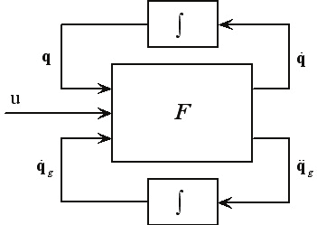
then it can be efficiently integrated according to the innovative integration scheme of Fig. 1,
where q& = & and F is a suitable function that allows computing q& and q& from u , q g
Bq
g
and q& .
g
Fig. 1. Block diagram for the robot forward dynamics integration.
Proof. It is easy to verify that the algorithm that describe the function F of the block scheme
of Fig. 1 is:
176
New Approaches in Automation and Robotics
Step 1. Compute (
B q) by applying one of the classic methods proposed in the literature (see
also Theorems 2 and 3 and (30) in Section 3).
Step 2. Compute q& through the relationship q& B 1−
=
q& .
g
Step 3. Compute (
c q, q&) and u .
a
d
Step 4. Compute
( q
B&) = q& = + γ +η +
+ .
g
c
ua u
dt
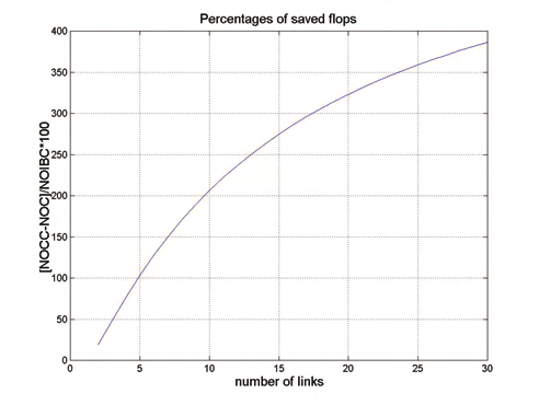
Remark 1. The proposed method allows avoiding the computation of the first term on the
right hand-side of (4) or of the first two terms on the right-hand side of (5). Such saving is
significant because the computational burden relative to this term is not negligible with
respect to the one required by the calculation of B−1 q& .
g
This clearly emerges from Fig. 2, where the percentages of saved flops vs. the number of
flops required to compute B 1− q& are evaluated (in MATLABTM environment) with reference
g
to the coefficients in (4), for a considerable number of cases of robots with random and
anyhow realistic links parameters.
Fig. 2. Percentages of saved flops evaluated for robot models with random links parameters.
Remark 2. Since many efficient algorithms for the numerical computation of the matrix B
are available in the literature, the gradient of the kinetic energy c can be computed in a very
simple and accurate way numerically, instead of using a symbolic expression.
To this end, since the kinetic energy for the majority of the robots is a quadratic function
respect to q& , whose coefficients are constant with respect to q or depend on q according to i
terms of the type sin( aq ϕ
+ , the following lemma is useful.
i
)
Lemma 1. The derivative of sin( aq can be numerically computed by a two [three] points
i )
formula:
d
sin[ (
a q + Δ
aq
⎡ d
sin[ (
a q + Δ
a q
i
])− sin[ ( − Δ
i
])⎤
i
])− sin(
sin( aq
sin( aq
(8)
i ) =
i ) =
i )
⎢
⎥
dq
Δ
dqi
2Δ
i
⎣
⎦
An Innovative Method for Robots Modeling and Simulation
177
with error:
1
Δ
2
e = − a
aχ Δ
2
e ≤ a
, χ ∈ ( q , q + Δ
i
i
)
2
sin( ) ,
2
2
2
(9)
2
⎡
1
Δ
⎤
2 3
3
e = − Δ a cos( aχ ), e ≤ a
, χ ∈ q − Δ, q + Δ
⎢
.
3
3
(
)⎥
⎣
6
6
i
i
⎦
Proof. See any numerical computation book.
In view of Lemma 1 it is possible to compute, with a prescribed maximum error, the
gradient of the kinetic energy starting from the numerical knowledge of the inertia matrix
B rather than using, as usually found in literature, complex analytical calculations of the
analytical expression of B . In details, for practical precision purposes, a good value of
T
∂
q
∂ can be obtained using a two [three] points formula with
−3
−4
Δ = 10 ÷ 10 [with
2
−
3
Δ = 10 ÷ 10− ] and evaluating n- 1 [2( n- 1)] times the inertia matrix B numerically.
3. Planar robot modeling
In the case of planar robots with revolute joints, theorems can be introduced and
demonstrated to provide a sufficiently simple and efficient method of expressing both the
inertia matrix and the gradient of the kinetic energy in a closed and elegant analytical form.
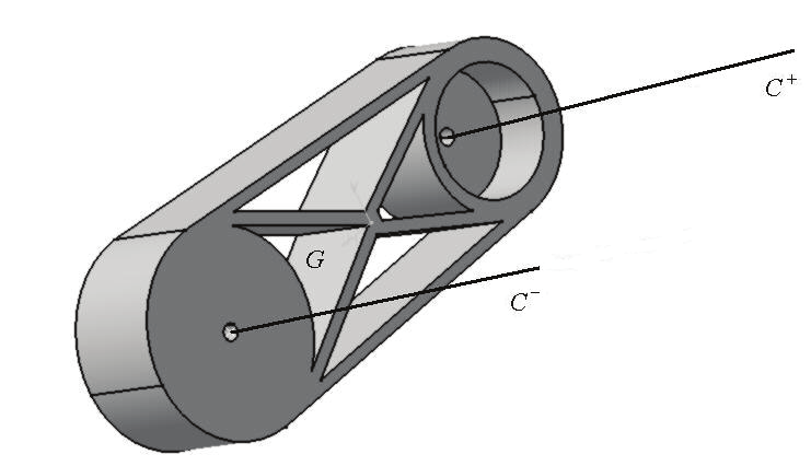
3.1 Hypotheses and notations
In the following it is considered the case of a generalised planar robot constituted by n links,
each of them with parallel rotation axes −
C , +
C and center of mass G belonging to the
plane containing the two relative rotation axes (see Fig. 3). In Fig. 4 a planar robot with three
links and a horizontal work plane is shown.
Fig. 3. The generic link of the considered generalised planar robot.
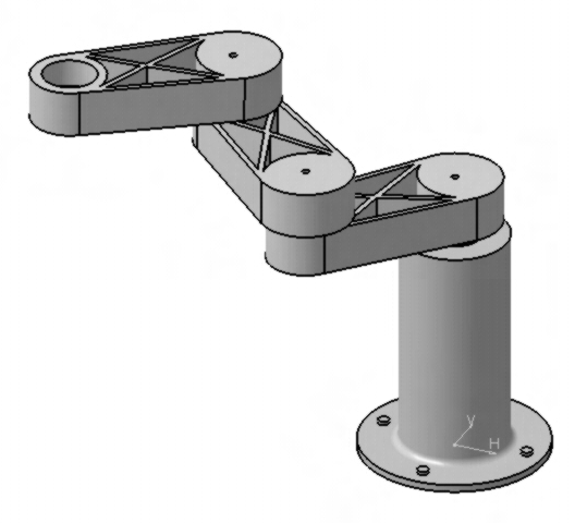
178
New Approaches in Automation and Robotics
Fig. 4. The considered generalised planar robot with three links and horizontal work plane.
Referring to Figs. 5 and 6 the next notations are also employed:
Y
Li
. +
C i
LGi
G i
.
α i
y i
−
C i
O
x i
X
Fig. 5. Geometric characteristics of the i-th link.
Y
L β
n
n α n
n
β4 α4
4
L 3β3
3
α3
L 2
2
β
L
α
2
1
1
2
β =α
1
1
X
Fig. 6. Schematic representation of a planar robot with n links.
An Innovative Method for Robots Modeling and Simulation
179
q =
T
[ x y α ] = absolute coordinates of the i-th link,
i
i
i
i
I
= inertia matrix of the i-th link in terms of the coordinates q ,
i
i
M
= total mass of the i-th link,
i
J , ρ = inertia moment and radius of the i-th link with respect to the rotation axis −
C ,
i
i
i
N
= static moment of the i-th link with respect to the plane containing −
C and
i
i
orthogonal to the plane passing through −
C and +
C ,
i
i
L
= distance of the center of mass G of the i-th link from the axis −
C ,
Gi
i
i
α =
T
[α α
α
= vector of the absolute angular coordinates of the chain constituted by
1
2 ...
]
1... i
i
the first i links,
<