Gi
if m i
and the notation h < k : var β , l = 2,K, i , indicates the set of the pairs h, k , with h < k , such l
that the angle α = α − α = β
+ β
+
between the links h and k varies with β .
1
2
... + β
hk
k
h
h+
h+
k
l
Proof. In view of Theorem 3, the kinetic energy of the generic i-th link is
1
2
2
1
2
~ ~
T = M ∑ L α& + M α& + M ∑ L L α& α&
α − α
i
i
h
h
i
i
i
h
k
h
k cos(
k
h )
2
h=1,.., i−1
2
h=1,.., i−1
k= h+1,.., i
~ ~
(32)
= T + M ∑ L L α& α&
α − α
c
i
h
k
h
k cos(
k
h ) ,
h=1,.., i−1
k= h+1,.., i
where T is the portion of kinetic energy that is independent of α
.
c
...
12 i
From (32) the expression (31a) of the gradient of Ti in terms of α
[ β
] easily follow.
12... i
12... i
The vector c can be simply obtained by suitably assembling the various vectors ci (i.e. by
progressively summing to the first i components of cn, i< n, the respective ci’s) .
In MATLAB-like instructions:
c=cn;
for i=n-1:-1:2
c(1:i)=c(1:i)+ci;
end.
Finally, it is important to note that if the work plane of the robot is vertical, the gravitational
torques can be calculated by using the following result.
Theorem 5. If the work plane of the robot is vertical, the weight of the i-th link originates a
torque on the k-th joint, k ≤ i :
i
γ = M g L~
∑ cosα ,
(33)
k
i
m
m
m= k
where g is the gravitational acceleration and the lengths L~ are given by (31b).
m
An Innovative Method for Robots Modeling and Simulation
185
Proof. The proof easily follows by considering Fig. 6.
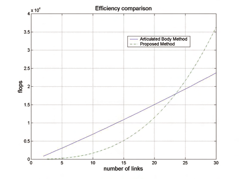
Remark 4. The proposed method efficiency has been explicitly compared to the Articulated
Body approach efficiency in terms of number of flops (in MatlabTM environment), for
executing the same elementary integration step by using the absolute Lagrangian
coordinates (see Fig. 9). From this figure it results that, for industrial robots with a limited
number of links, the proposed method is more efficient.
Fig. 9. Efficiency comparison between the Articulated Body method and the proposed
method.
Remark 5. The above-derived analytical expressions, in explicit form, of B , c and γ are
useful for speeding up the simulation, for comparing them to the proposed numerical
approach and for finally evaluating which terms can be simplified or neglected in the case of
robots with many and/or flexible links. Thus, for instance, for flexible link robots models,
obtained via discretization of the links, the terms relative to the deformation angles can be
simplified by substituting the sine function with the respective argument or even be
completely neglected, considering the terms relative to the motion only.
4. Spatial robot modeling
For spatial robots with generic shape links and connected, for the sake of brevity, with
spherical joints, several theorems are formulated and demonstrated in a simple manner
and some algorithms that allow computing in an efficient way analytically or numerically
both the inertia matrix and the gradient of the potential energy are provided.
4.1 Hypotheses and notations
In the following, for brevity, only spatial robots constituted by n links of generic shape,
connected by spherical joints are considered.
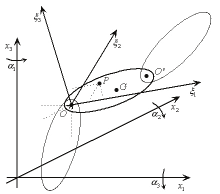
Moreover, the following notations will be used (see Fig. 10):
186
New Approaches in Automation and Robotics
Fig. 10. Coordinates of the generic point P of a link with respect to the body frame and to
the inertial frame.
q = [x T
α T ] T = [ x
x
x
α
α
α
= “absolute coordinates” of the i-th link,
i
O i
O i
i
i
i ] T
i
Oi
i
O 1
2
3
1
2
3
I = I
= inertia matrix of the i-th link with respect to the axes ξ , ξ , ξ ,
i
{ ihk}
1
2
3
ξ = ξ
[
ξ
ξ
= coordinates of the center of mass
i
G i
G i ] T
Gi
G 1
2
3
i
G in the body frame,
ξ
= ξ
= coordinates of the rotation center '
O in the body frame,
i
[
ξ
ξ
O i
O i
O i ] T
O '
'1
'2
'3
i
M = total mass of the i-th link,
i
α
=
= “angular absolute coordinates” of the chain constituted by the first i links,
i
[ T
T ... Ti ] T
1...
α1 α2
α
ℜ
= rotation matrix of the i-th link,
i (α i )
∂ℜ i(α i )
R =
,
ih
α
∂ ih
A = inertia matrix of the i-th link with respect to the coordinates α ,
i
1... i
α = α
= “absolute angular coordinates” of the robot,
1... n
A = inertia matrix of the robot with respect to the coordinates α ,
I = identity matrix of order 3,
shi = sin(α hi ) ,
chi = cos(α hi ) .
4.2 Main results
Let us consider a generic link of a generic shape of a spatial robot with spherical joints.
The following theorems and algorithms for the computation of the kinetic energy T of the i-
i
th link first as a function of the absolute coordinates q of the i-th link and then as a function
i
of the absolute angular coordinates α
of the chain constituted by the first i links are
1... i
provided.
Theorem 6. The kinetic energy of the i-th link may be calculated by means of the
relationship
An Innovative Method for Robots Modeling and Simulation
187
1
T = q T
& ℑ
i
i
iq
& ,
(34)
2
i
where
⎡
M I
M ∑ R ξ ⎤
i
i
hi Ghi
⎢
h
⎥
ℑ =
i
⎢
T
T
M ∑ R ξ
∑
.
(35)
R R I ⎥
i
hi Ghi
hi
ki hki
⎢
⎥
⎣
h
h , k
⎦
Proof. By omitting subscript i, the coordinates of the generic point P of the link in the fixed frame (see Fig. 10) are given by
x =
+ ℜ
,
(36)
P
x O
(α ξ
) P
where ℜ is the rotation matrix of the body frame with respect to the fixed frame and ξ is
P
the vector of the coordinates of the generic point P of the link in the body frame.
From (36) it follows
x& = & + ∑ R ξ
P
x O
h Phα
& ,
(37)
h
where
∂ℜ
R =
h =
.
(38)
h
,
1, 2, 3
α
∂ h
From (37) it is
2
V = x T
& x& = x T
T
T
& & + & ∑ R R ξ ξ & + & ∑ R ξ
h
k Ph Pk
2 T
P P
0 x0
α
α
x0
h Phα
& ,
(39)
h, k
h
from which
1
2
T =
V dm =
∫
2
1
T
1
=
x
T
T
T
M& & + & ∑ R R I & + M& ∑ R ξ & =
(40)
0 x0
α
h
k hkα
x0
h Ghα
2
2
h , k
h
⎡
MI
M∑ R ξ ⎤
1
= (
h Gh
⎢
⎥⎛ & ⎞
h
x
T
T
x&
α
0
0
& )
⎜ ⎟
2
⎢
T
T
M∑ R ξ
∑ R R I ⎥
h Gh
h
k hk
⎝ α& ⎠
⎢
⎥
⎣
h
h, k
⎦
and hence the proof.
Remark 6. The vector of the coordinates of the center of mass ξ iG and the inertia matrix
{ I of the i- th link, in the case of a complex structure, may be easily evaluated by making
hk }
use of software packages, such as CATIATM.
Theorem 7. If the Euler angles of the i- th link α = [
T
α
α
α
are the ZYX angles, also
i
1 i
2 i
3 i ]
called RPY angles ( Roll-Pitch-Yaw), (see Fig. 10), by omitting subscript i, the matrices Rh result:
188
New Approaches in Automation and Robotics
⎡− s c
− s s s − c c
− s s c + c s ⎤
1 2
1 2 3
1 3
1 2 3
1 3
R
⎢ c c
c s s
s c
c s c
s s ⎥
=
−
+
(41)
1
⎢ 1 2
1 2 3
1 3
1 2 3
1 3 ⎥
⎢ 0
0
0
⎥
⎣
⎦
⎡ c
− s
c c s
c c c ⎤
1 2
1 2 3
1 2 3
R
⎢ s s s c s s c c ⎥
= −
(42)
2
⎢ 1 2
1 2 3
1 2 3 ⎥
⎢ c
−
− s s
−
⎣
s c ⎥
2
2 3
2 3 ⎦
⎡0 c s c + s s
c
− s s + s c ⎤
1 2 3
1 3
1 2 3
1 3
R
⎢0 s s c c s
s s s
c c ⎥
=
−
−
−
. (43)
3
1 2 3
1 3
1 2 3
1 3
⎢
⎥
⎢0
c c
c
−
⎣
s
⎥
2 3
2 3
⎦
Proof. The rotation matrix ℜ
of the i- th link, by omitting subscript i, results (43)
i (α i )
⎡ c c
c s s − s c
c s c + s s ⎤
1 2
1 2 3
1 3
1 2 3
1 3
(α) ⎢ s c
s s s
c c
s s c
c s ⎥
ℜ
=
+
−
⎢
,
(44)
1 2
1 2 3
1 3
1 2 3
1 3 ⎥
⎢ −
⎣ s
c s
c c
⎥
2
2 3
2 3
⎦
from which, for (38), the proof.
The computation of the matrices ℑ may be sped up by the following algorithm, where
i
subscript i has been omitted.
Algorithm 1.
Step 1. Compute
1
s , s 2 , s 3; c 1, c 2 , c 3 .
(45)
Step 2. Compute
1
s s 2 , 1
s s 3, s 2 s 3;
c 1 c 2 , c 1 c 3, c 2 c 3;
s c , s c , s c ;
c s , c s , c s ;
1 2
1 3
2 3
1 2
1 3
2 3
(46)
( 1
s s 2) s 3, ( 1