k 1
+
b
z
+ b
z
+L+ b z
+ b
n 1
−
n 2
−
1
G ( z ) =
o
z
(3)
nk
nk 1
+
nk+ n 2
−
nk+ n 1
−
b z
+
o
1
b z
+L+ n
b −2 z
+ n
b 1
− z
The output signal of „FEEDBACK” corrector is formed as it follows: components of state
vector x(i) are passed through the transfer function ( Gz(z))-1. This creates auxiliary signals x’1(z) =[(Gz(z))-1 x1(z)], ...., x’n(z) = [(Gz(z))-1 xn(z)]. Then, on the basis of signals x’1(i) , ...., x’n(i) one can create signal uf(i) according to formula:
uf(i) = f [x’1(i –n k), x’2(i–(n–1) k),...,x’n(i –k)]
(4)
Note, that operation (4) processes the delayed signals x’1(i), ....,x’n(i). Next signal uf(i) has to be passed through the transmittance Gz(z). Its output signal is ufG(i). Finally, the output
signal Uf(i) of “FEDDBACK” corrector which “fits” for scheme shown in Fig. 2. is composed
using expression:
Uf(i) = ufG(i) - f[x1(i), x2(i), ..., xn-1(i) ] (5)
The input signal of structure shown in Fig.2 ought to be u(iT’), which means, that one has to
repeat the form of reference input signal of system shown in Fig. 1 (i.e. u(iT) for A-1 =α = 1), however the consecutive amplitudes of signal u(iT’) are changed now at moments ( iT’). Let
us note, that both systems (those in Fig. 1 and Fig. 2) operate with the same sample time T. If
order of denominator of Gz(z) is higher than order of nominator, then we can use function
G’z(z)=(zd G(z)) instead of G(z), where d represents the difference between denominator
order and nominator order. This “deviation” does not affect the form of output signal. It is
merely shifted forwards d samples T.
uA
y(iA-1T)
„INPUT”
(iT
+
CORRECTOR
SYSTEM
u(i A-1T)
+
x(iT)
Uf
„FEEDBACK”
CORRECTOR
Fig. 2. The time-scaling of linear and nonlinear SISO systems: u( iA-1T) - scaled reference
excitation, uA - system input scaling its response, y(iA-1T) - scaled reference response y(iT),
x(iT) - system state vector.
Example A. Let us consider the second order system (6) belonging to class (1):
x1(i+1) = x2(i)
x2(i+1) = f [ x1(i), x2(i) ] + u(i)
(6)
y(i) = F [b0 x1(i) + b1 x2(i) ]
where f (.) = - 0.72 x1(i) + 0.5 (x2(i))3 , F(.)= | 2 x1(i) + 5 x2(i)|.
336
New Approaches in Automation and Robotics
The response of system (6) to signal u(i) = 1 (i) for T = 1s is shown in Fig. 3. Let us assume, that form of that response fulfils the technical needs, however it is “too speedy” and should
be slowed down 2 times. Hence A= 0.5 , n=2, α = 2 k= 1 , b0= 2 , b1= 5 . Putting k= 1 , n= 2 to (3) one obtains the INPUT corrector (see Fig. 2) in the form:
2 +
5 z
2
G z (z) =
(7)
3
2
5 z + 2 z
To design FEEDBACK corrector we have to use (Gz(z))-1. Inversion of G(z) yields transfer
function with order of numerator higher than order of denominator. However, this is only
the apparent difficulty. Instead of G(z) we can put the invertible transfer functions Gz’(z) =
[ z Gz(z)] with identical orders of nominator and denominator to the FEEDBACK and INPUT
correctors . This “deviation” does not affect the form of output signal. It is merely shifted
forward one sample time period T.
y
8
uA 2
7
1.8
6
1.6
5
1.4
4
1.2
3
1
2
0.8
1
i
0.6
i
0
0.4
0
5
10
15
20
25
0
5
10
15
20
25
Fig. 3. Left position: the reference response of system (6) to signal u(i)= 1 (i) – curve
distinguished by “. ” - and response of system (6) obtained as output signal of structure in
Fig. 2 – curve distinguished by “o”. Note, that consecutive amplitudes of both responses are
identical (compare chosen referring amplitudes indicated by arrows). Right position:
reference input signal u(i) = 1 (i) and input signal uA(i) of system (6) when included to
structure in Fig. 2 as SYSTEM.
The FEEDBACK corrector (see Fig. 2) for system (6) and assumed values of A, k, n can be
defined by means of Gz’(z) =[ z G(z)] and nonlinear functions
uf(i) = f[x’1(i –2), x’2(i–1)] = - 0.72 x’1(i -2) + 0.5(x’2(i-1))3
Uf(i) = ufG(i) – f[x1(i), x2(i) ]
(8)
where signal ufG(i) is generated by passing of signal uf(i) through the transfer function
Gz’(z). The simulations carried out for structure like in Fig. 2 and data referring to current
example yield results shown in Fig. 3. We can observe, that described above algorithm
allows to design the INPUT and FEEDBACK correctors which guarantee the perfect result
of scaling.
Time-Scaling of SISO and MIMO Discrete-Time Systems
337
2.2 Speeding the system response up
Let model (1) be used for calculation of system input signal which speeds its reference
response up A times ( A - positive integer). If primary model (1) as well as system excitations
are defined for sample time T, then one cannot speed its response up without shortening of
sample time. We can treat, that operator z–1 associated with sample time T can be expressed
as z–1 = Z- A, where Z-1 refers to delay T’= A−1Τ. Thus, we can imagine, that each unit delay z –1 of “primary” structure in Fig. 1 is substituted by Z-A. The described transformations of
primary model (1) make, that modified structure operates with sample time T’, although
system model (1) has been defined for sample time T. Now, if we remove k = ( A-1) elements
Z–1 from each single “cell” z-1 = Z-A, then we obtain structure like in Fig. 1, where operators
z -1 are replaced with Z-1. If we put scaled signal u(iT’) to input of that modified structure (instead of primary u(iT)), then response of modified system will be speeded up A- times and
form of reference output (from before the described modification) will be conserved.
However, dealing with discrete-time models of real plants used for calculations of signals
for control purposes we cannot manipulate “inside” of structure modeling the plant and all
manipulations ought to be done “externally” in relation to plant model “interior”.
To solve the problem of scaling by synthesis of suitable input signal we can try to do
reconfiguration of modified structure like in Fig.1 (that containing Z –1 instead of z –1) to the
structure shown in Fig. 2, where SYSTEM represents the “primary” structure shown in Fig.1
from before modifications described above. Like in case taken into account in Section 2.1 the
current task can be solved similarly, due to equivalent transformations of modified structure
aimed at separation of its subsystem, which obtains the form of “primary” system, that
shown in Fig. 1, with unit delays z-1 replaced by chain of A single delays Z-1. The equivalent transformations are based on property Z–1 = z –1 Z k, where k = (A- 1). The calculations allow to define the following operation realized by “INPUT” corrector:
nk o
(n− )
1 k 2 A
k 2 (
A n− )
b Z Z + b Z
1
Z
+ .... + b − Z
1
Z
1
o
n
Gz(Z) =
(9)
k 1
+
(n− )(
1 k+ )
b
1
o + b Z
1
+ .... + bn− Z
1
The output signal of „FEEDBACK” corrector can be generated as it follows: the shifted
forward components of state vector, those corresponding to sample time T, i.e. x1(i+nk),
x2(i+(n–1)k),...,xn(i+k) should be passed through the transfer function ( Gz(Z))-1. This operation
yields the signals x’1(i+nk), x’2(i+(n–1) k),...,x’n(i+k) respectively. Using these auxiliary signals
one can form signal uf(i):
uf(i ) = f [x’1(i + n k), x’2(i+ (n–1) k),....,x’n(i +k)]
(10)
Note, that shifted forwards components of vector x are available, because they are generated
as output signals of “former” delay elements Z-1 creating chain of delays used for
assembling the model (1) or can be generated by delaying of “former” state variables
associated with model (1). Next signal uf(i) has to be passed through the transfer function
Gz(Z). Let output signal of Gz(Z) be denoted by ufG(i). Finally, the output signal Uf(i) of
“FEDDBACK” corrector (see Fig. 2) is composed using formula :
Uf(i) = ufG(i) - f[x1(i), x2(i), ..., xn-1(i) ] (11)
338
New Approaches in Automation and Robotics
The described rules allow to scale exactly the output y, if SYSTEM “pretends” operation
with sample time T (because of substitution z–1 = Z–A) and its real sample time is T’=( A-1T). It is obvious, that one cannot speed up the reference output y(iT), conserving its consecutive
amplitudes, if system sample time is still T. However, dependently of A, we can remove
every second, or every third, etc. amplitudes from reference sequence y(iT) and consecutive
remaining amplitudes generate with sample time T. This way can be treated as simplified
one for speeding the SYSTEM response up (some amplitudes of reference response are not
repeated), if sample time T of primary SYSTEM cannot be shortened. To obtain simplified
result of speeding of reference response up we can use signal uA (Fig. 2) which is generated
exactly like it was described above for SYSTEM operating with sample time T’. However,
signal uA determined for T’ should be passed through the “ZOH” (zero order hold) element
defined for sample time T. Then output signal of “ZOH” operation should be put as
excitation to input of “primary” SYSTEM, i.e. that operating with sample time T. It means,
that SYSTEM operating with T’ in structure like in Fig. 2 should be treated now as
calculation model of real primary SYSTEM operating with the sample time T.
Example B. Let us consider once more the second order system (6). The reference response
of system (6) to signal u(i) = 1 (i) for T =1 has been shown in Fig. 3. Let us assume, that form of considered response fulfills the technical needs, however it is “too slow” and should be
speeded up 2 times. Hence A= 2 , n= 2 , k= 1 , b0= 2 , b1= 5 . Putting k= 1 , n= 2 to (9) one obtains the INPUT corrector (see Fig. 2) in the form:
3
5 Z + 2
G z ( Z ) =
Z (12)
5
2
Z + 2
To avoid of processing of transfer function with higher order of nominator than order of
denominator we can use transfer function Gz’(Z) = [Z-1 Gz(Z)] with identical orders of
nominator and denominator. This “deviation” does not affect the form of time-scaled output
signal. It is merely shifted backwards one sample period T’. The FEEDBACK corrector (Fig.
2) for system (6) and assumed values A,k,n can be defined by means of Gz’(Z)=[Z-1 Gz(Z)]
and nonlinear functions:
uf(i)=f[x’1(i +2),x’2(i+1)]= - 0.72 x’1(i +2) + 0.5(x’2(i+1))3
Uf(i) = ufG(i) - f[x1(i), x2(i)]
(13)
where signal ufG(i) is generated by passing the signal uf(i) through the transfer function
Gz’(Z). The scheme of system for speeding the response of system (6) is shown in Fig. 4. The
exemplary simulation results are shown in Fig. 5.
The result of simplified scaling of system (6) is shown in Fig. 5 as well (see lowest position).
This result has been obtained by passing of signal uA generated in system shown in Fig. 4
through the “ZOH” operation defined for primary sample time T. After that, the output of
“ZOH” operation has been used as excitation of primary SYSTEM (6), that defined for
sample time T.
Time-Scaling of SISO and MIMO Discrete-Time Systems
339
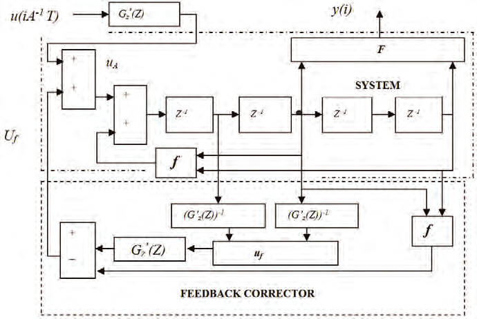
Fig. 4. The scaling of system (6) according to Fig. 2 and matter of Example B. Note, that
primary delays T (for z– 1) are substituted with the two delays T’ = 0.5 T, where T’ refers to operator Z –1.
2.3 Generalization
The considerations in previous Sections have been carried out for A being fraction with
numerator equal to one (for slowing the response down) or A being integer number (for
speeding the response up). The identical reasoning can be repeated, if each operator of
primary unit delay z-1 in system shown in Fig.1 is substituted with the chain of α operators
Z-1 associated with delay T’= T/α and next each single unit delay z-1=Z-α is substituted with ( Z- α Z-β ) for slowing the response or with ( Z- α Zβ ), where β < α , for speeding the response. All farther transformations aimed at separation of primary system structure (from
before scaling) can be done exactly like it has been described in previous Sections. Thus, it is
easy way of scaling if one needs to slow the response down [(α+β)/α] times or speed it up
[α/(α−β)] times. Of course, the obtained final structure (like in Fig. 2) has to be supplied with
scaled reference excitation u.
Looking for other possibilities of scaling of discrete-time systems we can adjust algorithms
for scaling of continuous-time systems (Durnas & Grzywacz, 2001; Durnas & Grzywacz,
2002; Grzywacz, 2006). The system (1) can be or can be treated as it would be the discrete-
time model of certain continuous-time system. So, one can determine the continuous–time
model associated with system (1). Then obtained model can be scaled like continuous-time
system. Finally, the respective scheme for scaling of continuous-time model can be
transformed back into discrete–time scheme. We must honestly admit, that scaling via
continuous-time representation does not guarantee the same consecutive amplitudes of
discrete-time output signals for variety of values of A. Nevertheless, we can treat this way
as determination of approximate solution.
340
New Approaches in Automation and Robotics
8
7
y
6
5
4
3
2
1
i
0 0
1
2
3
4
5
6
7
8
9
10
2.5
2
uA
1.5
1
0.5
0
-0.5
i
-1 0
1
2
3
4
5
6
7
8
9
10
8
y
7
6
5
4
3
2
1
i
0 0
1
2
3
4
5
6
7
8
9
10
Fig. 5. Upper figure: the reference response of system (6) to signal u(i)= 1 (i) - curve distinguished by “. ” - and the speeded response of system (6) obtained as output signal of
structure in Fig. 4 - curve distinguished by “o”. Note, that consecutive amplitudes of both
responses are identical (compare chosen referring amplitudes indicated by arrows). Below:
reference input u(i)= 1 (i) and input signal uA(i) of system (6) when included to structure in Fig. 4 (or in Fig. 2) as SYSTEM. The lowest position: the speeded response of system (6)
obtained as output of structure in Fig. 4 - curve distinguished by “o” - and simplified result
of scaling with sample time T - heavy line. Note, that every second amplitude of perfectly
scaled output y(iT’) is equal to respective amplitude of simplified result of scaling for
sample time T.
3. Time-scaling of MIMO systems
Let us assume, that MIMO system can be modelled by “V” structure (Chen, 1983) shown in
Fig. 6, where Vmj are linear or nonlinear operations processing the input or output signals
respectively. To scale the “V” structure one has to replace its SISO elements Vmj (Fig. 6) by
Time-Scaling of SISO and MIMO Discrete-Time Systems
341
respective SISO structures shown in Fig. 2 (where Vmj has to be treated as “SYSTEM” - see
Fig. 2 - and elements VImj, VFmj represent operations of associated INPUT corrector and
FEEDBACK one respectively). After the above modification of primary “V” structure one
can arrange the set of equivalent scheme transformations aimed at separation of primary
“V” structure. This goal can be achieved and signals uA1 , uA2 scaling the outputs y1 , y2 can
be generated by equipping the system with external correction loops. It means, that internal
structure of system is not affected. If the r