(35)
Where Λ
2
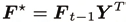
α= diag { α 2 , . . . , α
}
1
m is a diagonal matrix comprising squares of amplitude
constraints of u 1, t, . . . , u m, t on its diagonal.


366
New Approaches in Automation and Robotics
The amplitudes of elements of the control vector u t are constrained if the above LMI is
added to the set of LMIs (30)–(32).
The presented state-feedback control law stabilises the closed-loop system, guaranteed by
the existence of invariant ellipsoid describing V ( x t) with fully known plant and constant
reference vector.
In a similar manner, one can impose rate of changes constraints. If x t ≈ x t−1 is a state-vector of
approximately constant value, or in a steady-state, than
(36)
where F t−1 is a matrix computed at previous sample and F is the sought matrix computed at the current time instant.
As it has been stated in (Horla, 2007a), imposing symmetrical constraints on rates of
elements of u t is equivalent to imposing constraints on
(37)
where
should be a symmetrical matrix.
Assuming that
hold, one can obtain approximate rough rate
constraint as
(38)
or as LMI
(39)
where
is a diagonal matrix comprising squares of rate constraints
of u1, t, . . . , um, t on its diagonal.
The rates of elements of the control vector u t are constrained if the above LMI is added to the
set of LMIs (30)–(32).
8. Performance index, evaluation of directional change
Evaluation of control performance that is coupled with anti-windup compensation requires
following indices to be introduced:
(40)
(41)
(42)
Directional Change Issues in Multivariable State-feedback Control
367
(43)
where (40) corresponds to mean absolute tracking error of p outputs, (42) is a mean absolute
direction change in between computed and constrained control vector, and ϕ denotes angle
measure. In the case of m = 3, ϕ corresponds to absolute angle measure (in which case there
is no need to decide its direction).
9. Plant models for simulation studies
The considered plants are taken with delay d = 1 and are cross-coupled (values of control
offset have been given for reference signals of amplitude 3, where in the case of P3 the last
amplitude of reference signal is zero):
•
P1 ( m = 2, p = 2)
•
P2 ( m = 3, p = 2)
•
P3 ( m = 2, p = 3)
10. Simulation studies
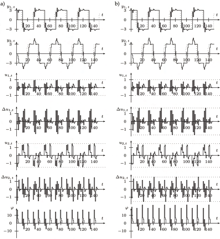
The performed simulations present anti-windup compensation performance for three
different plants and hard constraints imposed on the components of the control vector.
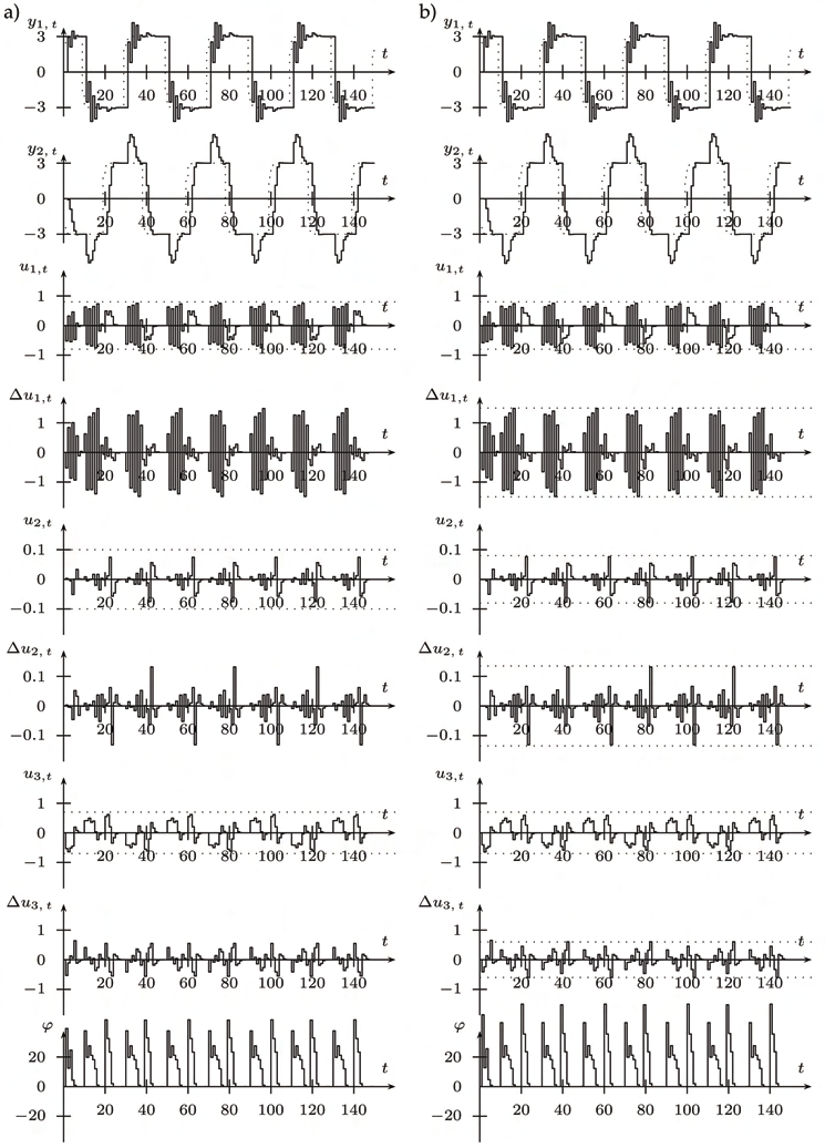
There are two systems simulated and depicted in the Figure 5, namely systemwith
amplitude constraints only and with added rate constraints, clipping only a part of the rates
of changes in order to enable a comparison. From Table 1 it is visible that for this case of
system with equal number of inputs and outputs, thus possible for dynamic decouplingwith
time-varying state-feedback control law, introducing additional constraints causes
performance indices to increase (i.e. there is more windup phenomenon in the system) and,
simultaneously it causes more severe directional change.
368
New Approaches in Automation and Robotics
This is because of the fact that one-step-ahead cannot foresee future changes of reference
signals, nor can assure perfect decoupling. Since imposed constraints alter the direction of
unconstrained control vector, directional change is necessary to alter the coupling in the
system, in order to achieve better control performance.
Fig. 5. P1: a) α 1 = 1.0, α2 = 1.5, β 1 = β 2 = ∞,
b) α1 = 1.0, α2 = 1.5, β1 = 1.7, β2 = 1.5)
Directional Change Issues in Multivariable State-feedback Control
369
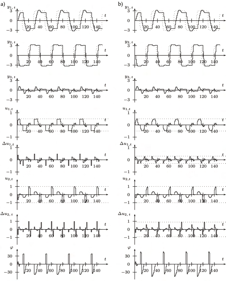
Fig. 6. P2: a) α1 = 0.8, α2 = 0.1, α3 = 0.7, β1 = β2 = β3 = ∞, b) α1 = 0.8, α2 = 0.1, α3 = 0.7, β1 = 1.5,
β2 = 0.14 , β3 = 0.6)
370
New Approaches in Automation and Robotics
Fig. 7. P3: a) α1 = 1.0, α2 = 1.5, β1 = β2 = ∞, b) α1 = 1.0, α2 = 1.5, β1 = 0.3, β2 = 0.9)
Directional Change Issues in Multivariable State-feedback Control
371
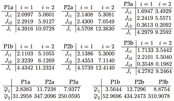
Table 1. Performance indices: a) without, b) with rate constraints
In the case of plant with greater number of control inputs than plant outputs (P2), Figure 6,
it is visible that in comparison with P1 the directional change is more severe, because of
three components of control vector changing in time. There are more degrees or freedom
(ways in which control vector may very in time, it varies in space to be exact, instead as
previously in plane), thus it is necessary to alter its direction in order to improve
decoupling. Once again performance indexes tend to increase with rate constraints added.
For the last plant considered, P3, it is obvious that since the number of control inputs is
deficient in comparison with plant outputs, direction of control vector corresponds to good
tracking performance, thus having introduced rate constraints it should not be altered
excessively. By comparison of directional change indices and performance indices for P3 it is
visible that by introducing rate constraints one can avoid bumps in control signals, what
leads to better tracking.
11. Concluding remarks
Solving the windup phenomenon problem does not have to mean that constrained control
vector is of the same direction as computed control vector if cross-coupling is present in the
control system. The presented state-feedback control law by avoiding generation of
infeasible control actions compensated windup phenomenon in a priori manner, though as
it can be seen, directional change is present in the system in order to assure better
decoupling.
On the other hand, avoiding directional change in control enables one to avoid windup
phenomenon if and only in the plant is perfectly decoupled or is not coupled at all. The
latter due to the constraints is hardly ever met, and if the application of some control law
does no require to preserve direction of control vector (what might correspond to, e.g.,
keeping proportions in between control signals), one should allow directional change to take
place. This will both improve anti-windup compensation performance and plant
decoupling.
372
New Approaches in Automation and Robotics
12. References
Albertos, P. and Sala, A. (2004). Multivariable Control Systems. Springer-Verlag, London,
United Kingdom.
Boyd, S., Ghaoui, L. E., Feron, E., and Balakrishnan, V. (1994). Linear Matrix Inequalities in
System and Control Theory. Society for Industrial and AppliedMathematics,
Philadelphia, United States of America, 3rd edition.
Boyd, S. and Vandenberghe, L. (2004). Convex Optimization. Cambridge University Press,
United Kingdom.
Doná, J. D., Goodwin, G., and Seron, M. (2000). Anti-windup and model predictive control:
Reflections and connections. European Journal of Control, 6(5):455–465.
Horla, D. (2004a). Anti-windup compensators (in Polish). Studies in Automation and
Information Technology, 28/29:35–52.
Horla, D. (2004b). Direction alteration of control vector and anti-windup compensation for
multivariable systems (in Polish). Studies in Automation and Information Technology,
28/29:53–68.
Horla, D. (2006a). LMI-based multivariable adaptive predictive controller with anti-windup
compensator. In Proceedings of the 12th IEEE International Conference MMAR, pages
459– 462, Miedzyzdroje.
Horla, D. (2006b). Multivariable state-feedback control with windup phenomenon
avoidance. In Proceedings of the 18th ICSS, pages 143–146, Coventry.
Horla, D. (2006c). Standard vs. LMI approach to a convex optimisation problem in
multivariable predictive control task with a priori anti-windup compensator. In
Proceedings of the 18th ICSS, pages 147–152, Coventry.
Horla, D. (2007a). Close-to-optimal adaptive multivariable state-feedback controller with a
priori anti-windup compensator. In Proceedings of the 13th IEEE IFAC International
Conference on Methods and Models in Automation and Robotics, pages 363–368,
Szczecin.
Horla, D. (2007b). Directional change and windup phenomenon. In Proceedings of the 4th
IFAC International Conference on Informatics in Control Automation and Robotics, pages
CD–ROM, Angers, France.
Horla, D. (2007c). Directional change for rate-constrained systems with anti-windup
compensation. In Proceedings of the 16th International Conference on Systems Science,
volume 1, pages 122–131, Wrocław.
Horla, D. (2007d). Optimised conditioning technique for a priori anti-windup compensation.
In Proceedings of the 16th International Conference on Systems Science, pages 132–139,
Wrocław, Poland.
Maciejowski, J. (1989). Multivariable Feedback Design. Addison-Wesley Publishing Company,
Cambridge, United Kingdom.
Öhr, J. (2003). Anti-windup and Control of Systems withMultiple Input Saturations: Tools,
Solution and Case Studies. PhD thesis, Uppsala University, Uppsala, Sweden.
Peng, Y., Vrančić, D., Hanus, R., and Weller, S. (1998). Anti-windup designs for
multivariable controllers. Automatica, 34(12):1559–1565.
Walgama, K. and Sternby, J. (1993). Contidioning technique for multiinput multioutput
processes with input saturation. IEE Proceedings-D, 140(4):231–241.
21
A Smith Factorization Approach to
Robust Minimum Variance Control of
Nonsquare LTI MIMO Systems
Wojciech P. Hunek and Krzysztof J. Latawiec
Institute of Control and Computer Engineering
Department of Electrical, Control and Computer Engineering
Opole University of Technology
Poland
1. Introduction
The minimum phase systems have ultimately been redefined for LTI discrete-time systems,
at first SISO and later square MIMO ones, as those systems for which minimum variance
control (MVC) is asymptotically stable, or in other words those systems who have ‘stable’
zeros, or at last as ‘stably invertible’ systems. The redefinition has soon been extended to
nonsquare discrete-time LTI MIMO systems (Latawiec, 1998; Latawiec et al., 2000) and
finally to nonsquare continuous-time systems (Hunek, 2003; Latawiec & Hunek, 2002),
giving rise to defining of new ‘multivariable’ zeros, i.e. the so-called control zeros. Control
zeros are an intriguing extension of transmission zeros for nonsquare LTI MIMO systems.
Like for SISO and square MIMO systems, control zeros are related to the stabilizing
potential of MVC, and, in the input-output modeling framework considered, are generated
by (poles of) a generalized inverse of the ‘numerator’ polynomial matrix (.)
B . Originally,
the unique, so-called T -inverse, being the minimum-norm right or least-squares left inverse
involving the regular (rather than conjugated) transpose of the polynomial matrix, was
employed in the specific case of full normal rank systems (Hunek, 2002; Latawiec, 2004). The
associated control zeros were later called by the authors ‘control zeros type 1’ (Latawiec,
2004; Latawiec et al., 2004), as opposed to an infinite number of ‘control zeros type 2’
generated by the myriad of possible polynomial matrix inverses, even those called τ - and
σ -inverses also involving the unique minimum-norm or least-squares inverses (Latawiec,
2004; Latawiec et al., 2005b). Transmission zeros, if any, are included in the set of control
zeros; still, we will discriminate between control zeros and transmission zeros. In the later,
new ‘inverse-free’ MVC design approach based on the extreme points and extreme
directions method (Hunek, 2007; Hunek & Latawiec, 2006), it was possible to design a pole-
free inverse of the polynomial matrix (.)
B so that no control zeros did appear. Well, except
when transmission zeros are present, in which case the extreme points and extreme
directions method does not hold. In the current important result of the authors, the Smith
factorization of the polynomial matrix (.)
B can lead to its pole-free inverse, when there are
no transmission zeros. Well, provided that the applied inverse is just the T -inverse, the
374
New Approaches in Automation and Robotics
intriguing result bringing us back to the origin of the introduction of control zeros. And in
case of any other inverse of Smith-factorized (.)
B we end up with control zeros.
The remainder of this paper is organized as follows. System representations are reviewed in
Section 2. Section 3 presents the problem of minimum variance control for discrete-time LTI
MIMO systems. Section 4 describes the new approach to MVC design, confirming the
Davison’s theory of minimum phase systems and indicates the role of the control zeros in
robust MVC-related designs. A simple simulation example of Section 5 indicates favorable
properties of the new method in terms of its contribution to robust MVC design. New
results of the paper are summarized in the conclusions of Section 6.
2. System representations
Consider an nu -input ny -output LTI discrete- or continuous-time system with the input
(
u t) and the output y( t) , described by possibly rectangular transfer-function matrix
G
ny × nu
∈R
( p) in the complex operator p , where p = z or p = s for discrete-time or continuous-time systems, respectively. The transfer function matrix can be represented in
the matrix fraction description (MFD) form (
G p)
−1
= A ( p) (
B p) , where the left coprime
polynomial matrices A
ny × ny
∈R
[ p] and B
ny × nu
∈R
[ p] can be given in form
n
A( p) = p I + ... + a
m
n and B( p) = p b +
0
... + bm , respectively, where n and m are the orders of
the respective matrix polynomials. An alternative MFD form
~
(
G p = (
~
) B p) −1
A ( p) , involving
right coprime ~
A
ny × ny
∈R
[ p] and ~
B
nu × ny
∈R
[ p] , is also tractable here but in a less
convenient way (Latawiec, 1998). Algorithms for calculation of the MFDs are known
(Rosenbrock, 1970; Wolowich, 1974) and software packages in the MATLAB’s Polynomial
Toolbox ® are available. Unless necessary, we will not discriminate between
−1
− n
A( p ) = I + ... + a
n
1
−
A p =
−1
−
(
) =
+ ... +
n p
and ( ) p
(
A p ) , nor between
m
B p
b
b
0
mp
and
(
B p) pm ( 1
−
=
B p ) . In the sequel, we will assume for clarity that (
B p) is of full normal rank; a
more general case of (
B p) being of non-full normal rank can be easily tractable (Latawiec,
1998). Let us finally concentrate on the case when normal rank of (
B p) is ny (‘symmetrical’
considerations can be made for normal rank nu ). Now, for discrete-time systems we have
−1
− n
− n
A( z ) = z A( z) = I + ... + a
−1
m
−
−
G( z) = −1
nz
and
m
B( z ) = z B( z) = b +...+ b
0
mz
, with
A ( z) (
B z) =
−
1
−
= z d A ( 1
−
z ) ( 1
−
B z ) , where d = n − m is the time delay of the system. The analyzed MFD
form can be directly obtained from the AR(I)X/AR(I)MAX model of a system
−
( 1
A q ) y( t) =
= q− d ( −1
B q ) (
u t) +[ C( 1
q− )/ ( −1
D q )] (
v t) , where −1
q is the backward shift operator,
ny
y( t)∈ R
,
n
n
u
u( t)∈R
and
y
v( t)∈ R
are the output, input and uncorrelated zero-mean disturbance,
respectively, in (discrete) time t ; A and B as well as A and C
ny × ny
∈ R
[ z] are relatively
prime polynomial matrices, with
−1
− k
C( z ) = c + ...+ c
0
k z
and k ≤ n , and the D polynomial in
A Smith Factorization Approach to Robust Minimum Variance Control of
Nonsquare LTI MIMO Systems
375
−1
z -domain is often equal to