New Approaches in Automation and Robotics by Harald Aschemann - HTML preview

0

− 1

⎢0

⎥

⎢

⎥

−1

−1

−1 ⎢

q

− 10 ⎥

⎢1 − 10 − 19 q

1 + 3 9

. q ⎥

⎣

⎦⎢0

0

⎥

(9)

⎣

⎦

⎡ 1

0⎤~−1

• ⎢

F ( −1

q

[

~

) y ( t +

⎥

d) − H( −1

q ) y( t)

ref

]

− 1 1

⎣

⎦

−1

1

−

with specific forms of ~

F ( 1

−

q ) and ~

H ( 1

−

q ) not presented here due to their mathematical

complexity. Now, for y 1

= 1

ref

, y 2

= 5

.

1

ref

the outputs remain at the setpoint for t ≥ d = 2

under the stabilizing perfect control, whose plots u 1( t) , u 2( t) and u 3( t) according to equation (9) are shown in Fig. 1. For clarity, we have chosen to show the performance of

(noise-free) perfect control rather than MVC.

3

2.5

2

1.5

u (t)

3

1

0.5

u (t)

1

0

u (t)

2

-0.50

2

4

6

8

10

12

14

16

18

20

t

Fig. 1. Perfect control plots for the specific example

Remark. However, the Smith factorization approach undeniably contributes to the robust

MVC design, in the majority cases the application of the control zeros can give much better

results (Hunek, under review), giving rise to the extension of the Davison’s theory of

minimum phase systems (Davison, 1983). Unfortunately, there exists no formal proof of the

above statement and it has been left for future research.

6. Conclusions

The Smith factorization approach to the robust minimum variance control has been

presented in this paper. The new method appears much better than others, designed by

A Smith Factorization Approach to Robust Minimum Variance Control of

Nonsquare LTI MIMO Systems

379

authors, namely those based on the extreme points and extreme directions method and

second one called minimum-energy. Firstly, it is computationally much simpler and

secondly, it works also for the case when transmission zeros are (nongenerically) present in

the nonsquare system. Strange enough, the presented method should operate on the T -

inverse exclusively and any other inverse applied gives rise to the appearance of control

zeros. What is also strange, applying the T -inverse directly to the polynomial (.)

B (rather

than to its Smith-factorized form) inevitably ends up with control zeros. Finally, the new

approach confirms the Davison’s theory and indicates the need of the introduction of the

complementary control zeros theory.

7. References

Davison, E. J. (1983). Some properties of minimum phase systems and 'squared-down'

systems. IEEE Trans. Auto. Control, Vol. AC-28, No. 2, 1983, pp. 221-222.

Desoer, C. A. & Schulman, J. D. (1974). Zeros and poles of matrix transfer functions and

their dynamical interpretation. IEEE Trans. Circuits & Systems, Vol. CAS-21, No. 1,

1974, pp. 3-8.

Hunek, W. P. (2003). Control zeros for continuous-time LTI MIMO systems and their application

in theory of circuits and systems (in Polish), Ph.D. thesis, Opole University of

Technology, Department of Electrical, Control and Computer Engineering, Opole.

Hunek, W. P. (2007). A robust approach to the minimum variance control of LTI MIMO

systems. Emerging Technologies, Robotics and Control Systems, Vol. 2, 2007, pp. 133-

138, ISBN: 978-88-901928-9-5; also in International Journal of Factory Automation,

Robotics and Soft Computing, Vol. 2, 2007, pp. 191-196, ISSN: 1828-6984.

Hunek, W. P. (to be published). Towards robust minimum variance control of nonsquare

LTI MIMO systems. Archives of Control Sciences.

Hunek, W. P. & Latawiec, K. J. (2006). An inverse-free approach to minimum variance

control of LTI MIMO systems, Proceedings of 12th IEEE International Conference on

Methods and Models in Automation and Robotics (MMAR’2006), pp. 373-378,

Międzyzdroje, Poland, August 2006.

Hunek, W. P. & Latawiec, K. J. (under review). Minimum variance control of discrete-time

and continuous-time LTI MIMO systems - a new unified framework. Control and

Cybernetics.

Kaczorek, T. (1998). Vectors and Matrices in Automatic Control and Electrical Engineering (in

Polish), WNT, Warszawa.

Latawiec, K. J. (1998). Contributions to Advanced Control and Estimation for Linear Discrete-Time

MIMO Systems, Opole University of Technology Press, ISSN: 1429-6063, Opole.

Latawiec, K. J. (2004). The Power of Inverse Systems in Linear and Nonlinear Modeling and

Control, Opole University of Technology Press, ISSN: 1429-6063, Opole.

Latawiec, K. J.; Bańka, S. & Tokarzewski, J. (2000). Control zeros and nonminimum phase

LTI MIMO systems. Annual Reviews in Control, Vol. 24, 2000, pp. 105-112; also in

Proceedings of the IFAC World Congress, Vol. D, pp. 397-404, Beijing, P.R. China, 1999.

Latawiec, K. J. & Hunek, W. P. (2002). Control zeros for continuous-time LTI MIMO

systems, Proceedings of 8th IEEE International Conference on Methods and Models in

Automation and Robotics (MMAR’2002), pp. 411-416, Szczecin, Poland, September

2002.

380

New Approaches in Automation and Robotics

Latawiec, K. J.; Hunek, W. P. & Adamek, B. (2005a). A new uniform solution of the

minimum variance control problem for discrete-time and continuous-time LTI

MIMO systems, Proceedings of 11th IEEE International Conference on Methods and

Models in Automation and Robotics (MMAR’2005), pp. 339-344, Międzyzdroje,

Poland, August-September 2005.

Latawiec, K. J.; Hunek, W. P. & Łukaniszyn, M. (2004). A new type of control zeros for LTI

MIMO systems, Proceedings of 10th IEEE International Conference on Methods and

Models in Automation and Robotics (MMAR’2004), pp. 251-256, Międzyzdroje,

Poland, August-September 2004.

Latawiec, K. J.; Hunek, W. P. & Łukaniszyn, M. (2005b). New optimal solvers of MVC-

related linear matrix polynomial equations, Proceedings of 11th IEEE International

Conference on Methods and Models in Automation and Robotics (MMAR’2005), pp. 333-

338, Międzyzdroje, Poland, August-September 2005.

Latawiec, K. J.; Hunek, W. P.; Stanisławski, R. & Łukaniszyn, M. (2003). Control zeros versus

transmission zeros intriguingly revisited, Proceedings of 9th IEEE International

Conference on Methods and Models in Automation and Robotics (MMAR’2003), pp. 449-

454, Międzyzdroje, Poland, August 2003.

Rosenbrock, H. H. (1970). State-space and Multivariable Theory, Nelson-Wiley, New York.

Wolowich, W. A. (1974). Linear Multivariable Systems, Springer-Verlag, New York.

22

The Wafer Alignment Algorithm

Regardless of Rotational Center

HyungTae Kim, HaeJeong Yang and SungChul Kim

Korea Institute of Industrial Technology

South Korea

1. Introduction

Semiconductor manufacturers prefer automatic machines due to quality, productivity and

effectiveness. Compared with other industries, the semiconductor industry has automized

the individual steps of a process to a relatively high level. Most of the operators usually

learn about wafer placement rather than the principle of the process. But the manual

systems do not know the placement of a wafer, so operators should set the initial conditions

for the process. Wafer alignment is an operation for correcting the current wafer position in

the system coordinate until the wafer is located at the target position. The wafer position

varies after loading, so alignment steps are required.

Manual alignment systems need the operators’ help every time the wafer is loaded and is

actually a time-consuming process, that lowers manufacturing productivity and raises costs.

So, automatic alignment can save these time and costs. If the machines have automatic

alignment function, wafer processes can be connected automatically. Operators then would

only have to check and monitor the processing situation, and fix a problem when it arises.

Therefore, one operator can operate more machines, and would not be required to have high

process skills. Fig. 1 shows the concept of wafer alignment in the dicing process.

Passive alignment is related with mechanical structures which persist into external forces

without any actuators. A self-constrained mechanism is developed by Choi. When axial

force is exerted on a stage, grooves beneath the stage generate internal stress which prevents

from moving the stage (Choi et al., 1999). Pyramid and groove mechanism make stacking

force under external stress (Slocum & Weber, 2003).

Active alignment skill using sensors and actuators is applied widely in semiconductor

manufacturing process. Anderson’s method (Anderson et al, 2004) is based on cross-relation

between a defined template and an inspected image. He segmented the pixels around a

peak and interpolated under sub-pixel level. Misalignment can be detected by Moire effect

and laser beam. PZT actuators are applied to remove misalignment in lithography (Fan et

al., 2006). Machine vision is a common device to detect misalignment in wafer aligment

(Hong & Fang, 2002).

We have developed an algorithm for wafer alignment. This alignment algorithm was

derived from rigid body transformation or object transformation. The algorithm was based

on the simultaneous motion of x-y-θ axes in 2D space. A 2-step algorithm has a simple

form which can be written by 2×2 matrix operations. The magnitude of misalignment was

382

Desktop\New Approaches in Automation and Robotics

reduced in base of macro and micro inspection data(Kim et al., 2004). The matrix was

expanded with 4×4, and θ was included in the equation. So, the alignment variables of x-y-

θcan be calculated within one equation(Kim et al, 2004), (Kim et al, 2006). The

manufacturing condition which was varied to be ideal conditions, affected the quality of

alignment. Sometimes the misalignment did not become zero after only macro-micro

alignment. In this case, the problem can be solved by iterative alignment equation, which is

similar to numerical algorithms(Kim et al, 2007). The convergence speed of the iteration can

be controlled by the convergence constant. This constant can prevent numerical vibration.

The convergence analysis method, similar to a numerical method, is proposed(Kim et al,

2006). We tried to obtain the exact solution in these studies, but they found that the solutions

can be obtained from an estimated equation. The idea in this study came from the estimated

method. The equation could be simplified by making a few assumptions of the wafer

alignment condition. The derived formula did not have the terms for rotational center,

which was impossible to measure exactly. The alignment results showed that the

performance of the proposed algorithm was similar to the exact solution, and that the error

convergence speed can be controlled.

Fig. 1. Concept of wafer alignment in dicing process

2. Review of 2D alignment model

2.1 Coordinate transformation for alignment(Kim et al, 2004)

The machine coordinate in the alignment system has three variables - x, y and θ. Let be the

P(x,y) original coordinate, and P’(x’,y’) be the transformed coordinate. The each coordinate

can be shown as follows

T

T

T

P = ( x y θ )

1

P′ = ( x′ y′ θ ′ )

1

P = C

(

C 0 0)

x

y

(1)

The Wafer Alignment Algorithm Regardless of Rotational Center

383

The alignment space is on 2D, the alignment procedure carries out translation and rotational

motion. The movement can be described by rigid body transformation and the coordinate

after the motion can be calculated simply by multiplying matrices. The notation of the

translational matrix usually has a ‘T’, the rotational matrix has an ‘R’ and the center of

rotation has a ‘C’. Then the transformation is formulated by equation (2).

P′ = T{ R( P − C) + C}

(2)

TR matrices in the wafer alignment system can be derived as equations (3) and (4), which

are 4 × 4 matrices.

⎡1 0 0 Δ x⎤

⎢

⎥

0 1 0 Δ y

⎢

⎥

T = ⎢

(3)

0 0 1 0 ⎥

⎢

⎥

⎣0 0 0 1 ⎦

⎡cos Δθ − sin Δθ 0 0 ⎤

⎢

⎥

sin Δθ cos Δθ 0 0

⎢

⎥

R = ⎢

(4)

0

0

1 Δθ ⎥

⎢

⎥

⎣ 0

0

0 1 ⎦

2.2 Basic alignment algorithm(Kim et al, 2006)

The wafer has marks for alignment. The ideal mark position Pt is stored when the wafer is

perfectly aligned. Misalignment is calculated from the current position Pc. The vision system

inspects the location of the mark on the screen. These mark positions can be defined as

follows.

T

T

P = ( x y θ

)

1

P = ( x y θ

)

1

t

t

t

t

c

c

c

c

(5)

When the current position of the mark is deviated from the ideal one, the resulting

displacement can be defined as 4. The mark position in the machine can be obtained from

the target position and the displacement by equation (6).

P ≈ P + Δ = (x + Δx, y + Δy, θ + Δθ, 1 T

)

(6)

c

t

c

c

c

If the current position is compensated with an arbitrary value α = (α x, α y, α , 0), the mark

θ

will be located at the target position. So, an alignment algorithm f(x) can be written by

equation (7).

f(P ,α) − P = 0

c

t

(7)

f(Pc,α) can be replaced with the equation from the rigid body transformation. The result is

shown as (8). The T and R have the unknown compensation variable for the current

position.

384

Desktop\New Approaches in Automation and Robotics

T{R(P − C) + C} − P = 0

c

t

(8)

The plus direction between the mathematical coordinate and vision can be reverse, and the

relation can be written by vision direction matrix Dv whose diagonal terms have a value of

either +1 or -1 and the other terms are zero.

T{R(P + D Δ − C) + C} − P = 0

t

v

t

(9)

The direction problem can occur between the math coordinate and the machine, and the

machine direction matrix Dm has the similar characteristics as Dv.

T

β = D α β = (β β β

)

1

m

x

y

θ

(10)

The unknown α can be calculated from the equation, and (11) and (12) are the exact solution

in the case when two points are inspected to align a line.

α = x -C -(x -C ) cos θ + (y -C ) sin θ

xn

tn

x

cn

x

n

cn

y

n

α

(11)

= y -C -(x -C ) sin θ -(y -C ) cos θ

yn

tn

y

cn

x

n

cn

y

n

(x − x )(y − y ) − (y − y )(x − x )

tan α

c 1

c 2

t 1

t 2

c 1

c 2

t 1

t 2

=

θ

(12)

(x − x )(x − x ) + (y − y )(y − y )

t 1

t 2

c 1

c 2

t 1

t 2

c 1

c 2

3. Centerless model

3.1 Simplification

The equations (11) and (12) are the exact solution, but estimated solutions have been used

for many numerical problems. Some variables can be erased by geometric relations and

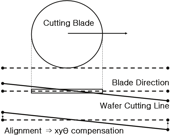
alignment conditions. Fig. 2 shows the general condition for wafer alignment in the dicing

process. First, angular misalignment in the process is within ±2o, which means sin α ≈ α and

cos α ≈ 1. the equation (11) can be written as follows

α = x -x + (y -C ) sin α = − Δ + (y -C )α

xn

tn

cn

cn

y

θn

xn

cn

y

θn

(13)

α = y -y -(x -C ) sin α = − Δ − (x -C )α

yn

tn

cn

cn

x

θn

yn

cn

x

θn

Second, inspection is carried out at two points, and the compensation value is the average,

α=(α1+α2)/2. And the inspection points are axis-symmetric at the rotational center,

2Cx−(xc1+xc2)=0. Another assumption is that the mark position is defined near the rotational

center, 2Cy−(yc1+yc2) = 0. Therefore, the equation (13) can be expressed as (14).

α = (

− Δ +