performance that it provides. In this phase, the controller for the configuration in figure 9 is
incorporated into the generalized plant G to form the system N , as shown in figure 11
w
N
z
Fig. 8. Relation between w and z in the generalized control problem.
It is relatively straightforward to show that the expression for N is given by
A Model Reference Based 2-DOF Robust Observer-Controller Design Methodology
15
1
N
G
G K (1 G K )−
=
+
−
G =& F ( G, K) (36)
11
12
22
21
l
where F denotes the lower Linear Fractional Transformation (LFT) of G and K . In order
l
to obtain a good design for K , a precise knowledge of the plant is required. The dynamics
of interest are modeled but this model may be inaccurate (this is usually the case indeed). To
deal with this problem the real plant P is assumed to be unknown but belonging to a class
of models built around a nominal model P . This set of models is characterized by a matrix
o
Δ , which can be either a full matrix (unstructured uncertainty) or a block diagonal matrix
(structured uncertainty), that includes all possible perturbations representing uncertainty to
the system. Weighting matrices W and W are usually employed to express the uncertainty
1
2
in terms of normalized perturbations in such a way that Δ
≤ 1 . The general control
∞
configuration in figure 9 may be extended to include model uncertainty as it is shown in
figure 9
D
w 1
z 1
w 2
z 2
G
u
v
K
Fig. 9. Generalized control problem configuration.
The block diagram in figure 9 is used to synthesize a controller K . To transform it for
analysis, the lower loop around G is closed by the controller K and it is incorporated into
the generalized plant G to form the system N as it is shown in figure 10. The same lower
LFT is obtained as if no uncertainty was considered.
D
w 1
z 1
w 2
z 2
N
Fig. 10. Generalized block diagram for analysis in the face of uncertainty.
To evaluate the relation from = [
T
w
w
w
to = [
] T
z
z
z
for a given controller K in the
1
2 ]
1
2
uncertain system, the upper loop around N is closed with the perturbation matrix Δ . This
results in the following upper LFT:
1
F (N , ) & N
N
(1 N
)−
Δ =
+
Δ −
Δ N
u
(37)
22
21
11
12
and so z = F (N , Δ) w . To represent any control problem with uncertainty by the general
u
control configuration it is necessary to represent each source of uncertainty by a single
16
New Approaches in Automation and Robotics
perturbation block Δ , normalized such that Δ
≤ 1 . We will assume in this work that we
∞
can collect all the sources of uncertainties into a single full (unstructured) matrix Δ .
3.2 Uncertainty and robustness
As already commented, an exact knowledge of the plant is never possible. Therefore, it is
often assumed that the real plant, denoted by P , is unknown but belonging to a set of class
models characterized somehow by Δ and with centre P .
o
Definition 4 (Nominal Stability) The closed-loop system of figure 9 has Nominal Stability
(NS) if the controller K internally stabilizes the nominal model P ( Δ = 0 ), i.e., the four
o
transfer matrices N , N , N , N in the closed-loop transfer matrix N shown in figure
11
12
21
22
13 are stable.
Definition 5 (Nominal Performance) The closed-loop system of figure 12 has Nominal
Performance (NP) if the performance objectives are satisfied for the nominal model P , i.e.,
o
N
< 1in figure 10 assuming Δ = 0 .
22 ∞
Definition 6 (Robust Stability) The closed-loop system has Robust Stability (RS) if the
controller K internally stabilizes the closed-loop system in figure 9 ( F (N , Δ) ) for every
u
Δ such that Δ ≤ 1 .
∞
We will just consider in this work additive uncertainty, which mathematically is expressed
as
P = { P : P = P + W Δ (38)
A
o
1 }
Being w a scalar frequency weight and Δ
≤ 1 . Now that we know how to describe the
A
∞
set of plants which our real plant is supposed to lie in the next issue is to answer the
question of when a controller stabilizes all the plants belonging to this set.
Theorem 5 (Robust Stability for unstructured uncertainty) Let us assume that we have
posed our system in the form illustrated by figure 9. The overall system is robustly stable
(see definition 6) iff
N
≤ 1
11
(39)
∞
where N has been defined in (36), see figure 10.
Robust stability conditions for the different uncertainty representations can be derived by
posing the corresponding feedback loops as in figure 9 and then applying theorem 5, also
known as the small gain theorem. See (Morari and Zafirou, 1989) for details.
4. The design for the proposed robust 2-DOF Observer-Controller
In this section a methodology for designing 2-DOF controllers is provided. The design is
based on the Observer-Controller configuration described in section 2.2. In order to have a
2-DOF scheme a prefilter block ( K ) has been added, leading to the general scheme shown
2
in figure 11
A Model Reference Based 2-DOF Robust Observer-Controller Design Methodology
17
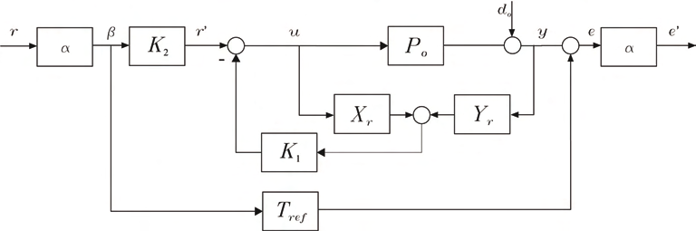
Fig. 11. The proposed 2-DOF control configuration.
The controller blocks X , Y , K which implicitly fix the Youla parameter Q of theorem 5
r
r
1
y
will be in charge of providing robust stability and good output disturbance rejection. On the
other hand, the prefilter K (the Youla parameter Q of theorem 5) has to cope with the
2
r
tracking properties of the system by solving a model matching problem with respect to a
specified reference model which describes the desired closed-loop behaviour for the
resulting controlled system.
4.1 Step I: Design of the Observer-Controller part through direct search optimization
In section 2.2 we characterized the Observer-Controller configuration in terms of the
polynomials p , p and m . Let us assume without loss of generality that additive output
K
L
uncertainty (38) is considered. In this first step of the design the objective will be to find
convenient p , p , m , defining entirely X , Y , K in figure 12. This search will be K
L
r
r
1
performed in order to provide robust stability with the best possible output disturbance
rejection.
Fig. 12. Observer-Controller part with additive uncertainty.
More specifically, for the scheme in figure 12 the following relations hold
u
⎡ ⎤ ⎡
M
− RM Y
M R
r (1
r )
⎤ ⎡ d ⎤
r
r
o
=
⎢
(40)
⎣ ⎥ ⎢
⎥ ⎢ ⎥
y '⎦
W
− N
− RM Y
N R
⎣
⎦ ⎣ r
p (1
r (1
r )
)
⎦
r
r
'
18
New Approaches in Automation and Robotics
where all the terms have been defined in section 2.2. It can be proved by applying theorem 5
to figure 12 (once put in the generalized controller configuration of figure 9) that robust
stability of the system in figure 12 amounts to satisfy the following inequality
T
≤ 1
u ' d
(41)
o
∞
The design for the Observer-Controller part reduces finally to solving the following
optimization problem
min
W
− N
− RM Y
p (1
r (1
r ) r )
p , p , m
∞
K
L
(42)
subject to
W M 1 − RM
Y
≤ 1
1 (
r (
r ) r ) ∞
Direct search techniques - see (Powell, M., 1998) - are suggested for solving the problem (42).
Basically they consist of a method for solving optimization problems that does not require
any information about the gradient of the objective function. Unlike more traditional
optimization methods that use information about the gradient or higher derivatives to
search for an optimal point, a direct search algorithm searches a set of points around the
current point, looking for one where the value of the objective function is lower than the
value at the current point. At each step, the algorithm searches a set of points, called a mesh,
around the current point—the point computed at the previous step of the algorithm. The
mesh is formed by adding the current point to a scalar multiple of a set of vectors called a
pattern. If the pattern search algorithm finds a point in the mesh that improves the objective
function at the current point, the new point becomes the current point at the next step of the
algorithm. In (Henrion, D., 2006) a recent application of direct search techniques for solving
a specific control problem can be consulted.
4.2 Step II: Design of the prefilter controller K
2
In this section we tackle the second step of our design. This step is aimed at designing a
prefilter controller for meeting tracking specifications given in terms of a reference model. In
order to achieve this goal a model matching problem is posed as in figure 13
Fig. 13. Model-matching problem arrangement for the design of K .
2
A Model Reference Based 2-DOF Robust Observer-Controller Design Methodology
19
where T is the specified reference model for the closed-loop dynamics. The idea is to
ref
make use of the general control framework introduced in section 3 and design K so as to
2
minimize the relation from r to e in an H sense. In doing so, we also want to have certain
∞
control over the amount of control effort employed to make the close loop resemble the
model reference. The parameter a will precisely play the role of enabling one to arrive at a
compromise between the tracking quality and the amount of energy demanded by the
controller, accommodating into the design this practical consideration.
Note that in the nominal case, i.e., P = P , the prefilter controller K sees just N R .
o
2
r
Therefore, the relation from the reference to the output reads as
y = N RK r
r
(43)
2
It should be noted that the N and R have already been fixed as a result of applying the first
r
step of the design. To include different and independent dynamics for the step response, we
have to take advantage of the second degree of freedom that K provides. From the overall
2
scheme in figure 11 we can compute the transfer matrix function that relates the inputs
[
T
d
r ] T , i.e., the disturbance d and the command signal r , with the outputs [ u '
e] ,
o
o
i.e., the weighted control signal u ' and the weighted model matching error e .
u '
W
−
1 − M ( X + RN Y )
W
a
M
1 − RM Y K
⎡ ⎤ ⎡ 1 (
r
r
r r )
1
r (
r )
⎤ d
⎡ ⎤
r
2
o
=
⎢ ⎥ ⎢
⎥ ⎢ ⎥ (44)
⎣ e ⎦
N
X + RN Y
a
N RK − T
⎣
r (
r r )
2 ( r
⎦ ⎣ ⎦
2
ref )
r
The H -norm of the complete transfer matrix function (44) is minimized to find K without
∞
2
modifying neither the robust stability margins nor the disturbance rejection properties
provided by the Observer Controller in the first step of the design. The 2-DOF design
problem shown in figure 13 can be easily cast into the general control configuration seen in
section 3. Comparing figures 12 and 13 with figure 9 we make the following pairings
w = d , w = r , z = u ' , z = e ' , v = b, u = u and K = K . The augmented plant G and 1
o
2
1
2
2
the controller K are related by the following lower LFT:
2
1
F ( G, K ) & G
G K (1 G K )−
=
+
−
G (45)
l
2
11
12
2
22
2
21
The corresponding partitioned generalized plant G is:
u '
d
⎡ ⎤
⎡ o ⎤
⎢ ⎥
⎡ 11
G
12
G
⎤ ⎢ ⎥
e '
=
r
⎢ ⎥
⎢
⎥
G
⎢ ⎥
⎣ 21
2
G 2 ⎦
⎢b⎥
⎢ r ' ⎥
⎣ ⎦
⎣ ⎦
(46)
⎡ W
−
− M X + RN Y
W M R⎤ d
1 (1
(
)
r
r
r r )
0
1
r
⎡ o ⎤
⎢
⎥ ⎢ ⎥
=
⎢
N
X + RN Y
−a T
a N R
r
r (
r
r r )
2
ref
r
⎥ ⎢ ⎥
⎢
⎥ ⎢ r '
0
a
0
⎥
⎢⎣
⎥ ⎣ ⎦
⎦
20
New Approaches in Automation and Robotics
Remark. The reference signal r must be scaled by a constant W to make the closed-loop
r
transfer function from r to the controlled output y match the desired reference model T
ref
exactly at steady-state. This is not guaranteed by the optimization which is aimed at
minimizing the H -norm of the error. The required scaling is given by
∞
W
( K (0) N (0) R(0) −
=&
T
(47)
r
) 1 (0)
r
2
ref
Therefore, the resulting reference controller is K W .
2
r
5. Illustrative example
In this section we apply the methodology presented in section 4 for designing a 2-DOF
controller according to figure 11 for the following nominal plant
5( s + 1.3)
P =
(48)
o
( s + 1)( s + 2)
The uncertainty in the model is parameterised using an additive uncertainty description as
in (38) with
3( s + 1)
W =
(49)
1
( s + 20)
Now we initialize the optimization problem (42) with the values
p = [−10 −10] T , p = [−20 −20] T , m = [1 2] T , where p ( p ) contains the initial Ko
Lo
o
K 0
L 0
roots of the polynomials p ( p ) and m the initial coefficients for the polynomial m .
K
<