1
y 2 y 1 y 2 ⎤⎦ . (32)
⎣q⎦
The equations of motion (9) are available in symbolic form. Inserting the muscle force
characteristics, the internal muscle pressures as control inputs can be parameterized by the
flat outputs and their time derivatives
⎡ p
M 1 l(q, q, q, pM 1 ) ⎤
⎢ p
⎥
⎢
M r (q, q, q, pM )
1
1 ⎥
u =
= (
u q, q, q, pM 1, pM 2 )
⎢
. (33)
p
q q q
⎥
M 2 l( , , , pM 2 )
⎢
⎥
⎢ p
⎣
M 2 r (q, q, q, pM 2 )⎥⎦
In the following, three different nonlinear control approaches are employed to stabilize the
error dynamics of the outer control loop: flatness-based control, backstepping and sliding-
mode control (Khalil, 1996). For all these alternative designs, the differential flatness
property proves advantageous (Sira-Ramirez & Llanes-Santiago, 1995; Aschemann et. al.,
2007).
3.3 Flatness-based control
In the case of flatness-based control, the inverse dynamics is evaluated with the measured
crank angles and the corresponding angular velocities obtained by real differentiation
(Aschemann & Hofer, 2005). For the mean pressures, however, desired values are utilized.
The second derivatives of the crank angles, the angular accelerations, serve as stabilizing
inputs
T
u = ⎡ p
⎣ M 1 l pM 1 r pM 2 l pM 2 r ⎤ = (
u q, q, v
⎦
1 , v 2 , pM 1 d , pM 2 d ) . (34)
The inverse dynamics leads to a compensation of all nonlinearities. An asymptotic
stabilization is achieved by pole placement with Hurwitz-polynomials for the error
dynamics for each drive i = {1, 2}
Nonlinear Model-Based Control of a Parallel Robot Driven by Pneumatic Muscle Actuators
35
t
v
i = qid + α i 2 ⋅ ( qid − qi ) + α i 1 ⋅ ( qid − qi ) + α
∫ i 0 ⋅( qid − qi) dτ . (35)
0
3.4 Backstepping control
The first step of the backstepping control design (Khalil, 1996) involves the definition of the
tracking error variable for each drive i = {1, 2},
e
i 1 = qid − qi
⇒ ei 1 = qid − qi . (36)
Next, a first Lyapunov function Vi 1 is introduced
!
1
2
2
i
V 1( ei 1) = ei 1 > 0 ⇒
1
V ( ei 1) = ei 1 ⋅ ei 1 = ei 1 ⋅( qid − qi)=− c 1 ⋅ ei 1 (37) 2
and the expression for its time derivative is solved for the virtual control input
e
i 1 = qid − qi = c
− 1 ⋅ ei 1 ⇒ qi ≈ α iI( ei 1, qid) = qid + c 1 ⋅ ei 1 . (38) In the second step, the error variable ei 2 is defined in the following form
e
i 2 = α iI ( ei 1 , qid ) − qi = qid − qi + c 1 ⋅ ei 1
⇒ ei 1 = ei 2 − c 1 ⋅ ei 1 (39)
and its time derivative is computed
e
i 2 = qid − qi + c 1 ⋅ ei 1 = qid − qi + c 1 ⋅ ( ei 2 − c 1 ⋅ ei 1 ) . (40) Now, a second Lyapunov function Vi 2 is specified.
1
1
2
2
i
V 2( ei 1, ei 2) = ei 1 + ei 2 > 0 ⇒
i
V 2( ei 1, ei 2 ) = ei 1 ⋅ ei 1 + ei 2 ⋅ ei 2 (41)
2
2
The corresponding time derivative
!
2
2
2
i
V 2( ei 1, ei 2 ) = c
− 1 ⋅ ei 1 + ei 2 ⋅[ qid − vi + c 1 ⋅( ei 2 − c 1 ⋅ ei 1) + ei 1]=− c 1 ⋅ ei 1 − c 2 ⋅ ei 2 (42) can be made negative definite by choosing the stabilizing control input as follows
2
v = q = q + e 1 ⋅(1 − c 1 ) + e 2 ⋅( c 1 + c 2)
i
i
id
i
i
. (43)
Backstepping control design offers several advantages in comparison to flatness based
control. It becomes possible to avoid cancellations of useful, i.e. stabilizing nonlinearities.
Furthermore, different positive definite functions can be used at control design, e.g.
allowing for nonlinear damping.
3.5 Sliding-mode control
For sliding-mode control (Sira-Ramirez & Llanes-Santiago, 1995) the vector of tracking
errors is considered
⎡ q − q ⎤
id
i
z i = ⎢
. (44)
q
⎥
⎣
id − qi ⎦
36
New Approaches in Automation and Robotics
Based on this error vector z i , the following sliding surfaces si are defined for each drive
i = {1, 2}
si(z
i ) = qid − qi + β i 1 ⋅ ( qid − qi ) ⇒
si = qid − qi + β i 1 ⋅( qid − qi) , (45)
where β i 1 represents a positive gain. The convergence to the corresponding sliding surface is
achieved by introducing a discontinuous switching function in the time derivative of a
quadratic Lyapunov function
1
2
i
V ( si ) = si ⇒
i
V ( si) = si ⋅ si ≤ α
− i| si|= α
− i ⋅ si ⋅ sig (
n si) , (46)
2
with a properly chosen coefficient α i that dominates remaining model uncertainties. The
control design offers flexibility as regards the choice of the sliding surfaces and the reaching
laws. For the implementation, however, a smooth switching function is preferred to reduce
high frequency chattering. This results in the following stabilizing control law, which leads
to a real sliding mode within a boundary layer
s
i
v
i = qi = qid + β i 1 ⋅ ( qid − qi ) + α i ⋅ tanh(
) . (47)
ε
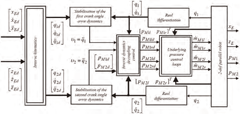
The implemented control structure is depicted in Fig. 8. The desired trajectories are
provided from an offline trajectory planning module that calculates time optimal trajec-
tories according to both state constraints and input constraints. This is achieved by proper
time-scaling of polynomial functions with free parameters as described in (Aschemann &
Hofer, 2005).
Fig. 8. Implementation of the decoupling control structure.
4. Disturbance observer design
The observer provides a vector ˆx2 of estimated disturbance torques that accounts for both
model uncertainties and nonlinear friction. The main idea consists in the extension of the
system state equations with the measurable state vector
Nonlinear Model-Based Control of a Parallel Robot Driven by Pneumatic Muscle Actuators
37
y x1 [q, q] T
=
=
(48)
by two integrators, which serve as disturbance models (Aschemann et. al., 2007)
y = f(y, ˆx , u), dim(y) = 4,
2
ˆx
(49)
= 0, dim(ˆ
2
x2 ) = 2.
The reduced-order disturbance observer according to (Friedland, 1996) is given by
z = Φ(y, ˆx , u), dim(z) =
2
2,
η
⎡ ˆ ⎤
ˆ
(50)
x = ⎢ 1
2
⎥ = H y + z ,
η
⎣ ˆ2 ⎦
where H denotes the observer gain matrix and z the observer state vector. The observer gain
matrix is chosen as follows
⎡ h
h
0
0 ⎤
11
11
H = ⎢
, (51)
0
0
h
⎥
⎣
22
h 22 ⎦
involving only two design parameters h 11 and h 22. Aiming at an asymptotically stable
observer dynamics
!
lim e = lim(x − ˆ
2
x2 )=0 , (52)
t→∞
t→∞
the observer gains are determined by pole placement based on a linearization using the
corresponding Jacobian (Friedland, 1996). In Fig. 9 a comparison of simulated disturbance
forces and the observed forces provided by the proposed disturbance observer is shown.
Here, the resulting tangential force at the pulley with radius r is depicted, which is related to
the disturbance torque according to F =ηˆ
iU
i / r . Obviously, the simulated disturbance
forces are reconstructed with high accuracy.
100
100
actual disturbance F2U
observed F2U
]
50
]
50
orce [N
orce [N
0
0
ial f
ial f
nt
nt
nge
nge
ta
-50
ta
-50
actual disturbance F1U
-100
observed F1U
-100
0
5
10
15
0
5
10
15
t [s]
t [s]
Fig. 9. Comparison of simulated disturbance force and observed disturbance force using the
reduced-order disturbance observer.
38
New Approaches in Automation and Robotics
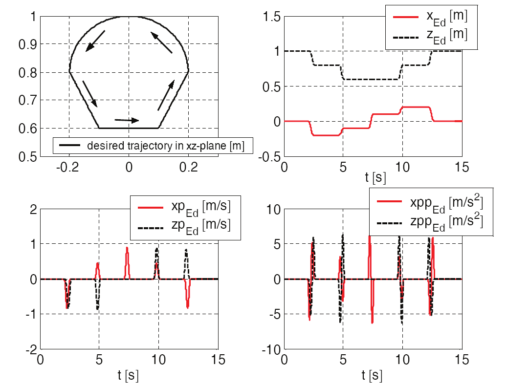
5. Simulation results
The efficiency of the proposed cascade control structure is investigated using the desired
trajectory shown in Fig. 10 with maximum velocities of approx. 0.9 m/s and maximum
accelerations of approx. 7 m/s2 for each axis.
The first part of the desired trajectory involves the motion on a quarter-circle with the radius
0.2 m from the starting point ( x = 0 m, z = 1 m) to the point ( x = −0.2 m, z = 0.8 m). The next three movements consist of straight lines: the second part comprises a diagonal movement
in the xz-plane to the point ( x = −0.1 m, z = 0.6 m), followed by a straight line motion in x-
direction to the point ( x = 0.1 m, z = 0.6 m). The fourth part is given by a diagonal movement
to the point ( x = 0.2 m, z = 0.8 m). The fifth part involves the return motion on a quarter-
circle to the starting point ( x = 0 m, z = 1 m).
Fig. 10. Desired trajectory in the workspace.
5 x 10⁻³
5 x 10⁻³
FB
BS
FB
0
]
]
SM
[m
0
[m
-5
e x
SM
e z
BS
-10
BS
-5
-15
0
5
10
15
0
5
10
15
t [s]
t [s]
Fig. 11. Comparison of the tracking errors in the workspace without disturbance observer.
Nonlinear Model-Based Control of a Parallel Robot Driven by Pneumatic Muscle Actuators
39
Fig. 11 shows a comparison of the resulting tracking errors in the workspace for flatness-
based control (FB), backstepping control (BS) and sliding-mode control (SM). Without
observer-based disturbance compensation, the best results are obtained using sliding-mode
control.
The efficiency of the observer based disturbance compensation is emphasized by Fig. 12. For
all considered control approaches a further improvement of tracking accuracy is achieved.
6. Conclusion
In this contribution, a cascaded trajectory control based on differential flatness is presented
for a parallel robot with two degrees of freedom driven by pneumatic muscles. The
modelling of this mechatronic system leads to a system of nonlinear differential equations of
eighth order. For the characteristics of the pneumatic muscles polynomials serve as good
approximations. The inner control loops of the cascade involve a flatness-based control of
the internal muscle pressure with high bandwidth. For the outer control loop three different
control approaches have been investigated leading to a decoupling of the crank angles and
the mean pressures as controlled variables. Simulation results emphasize the excellent
closed-loop performance with maximum position errors of approx. 1 mm during the
movements, vanishing steady-state position error and steady-state pressure error of less
than 0.03 bar, which have been confirmed by first experimental results at a prototype
system.
1 x 10⁻³
1.5 x 10⁻³
FB
1
0.5
]
SM
]
0.5
[m
0
[m
e x
e z
SM
0
-0.5
BS
FB
-0.5
BS
-1
-1
0
5
10
15
0
5
10
15
t [s]
t [s]
Fig. 12. Tracking errors in the workspace with observer-based disturbance compensation.
7. References
Aschemann H.; Hofer E.P. (2004). Flatness-Based Trajectory Control of a Pneumatically Driven
Carriage with Uncertainties, CD-ROM-Proc. of NOLCOS, pp. 239 – 244, Stuttgart,
September 2004
Aschemann H.; Hofer E.P. (2005). Flatness-Based Trajectory Planning and Control of a Parallel
Robot Actuated by Pneumatic Muscles, CD-ROM-Proc. of the ECCOMAS Thematic
Conference on Multibody Dynamics, Madrid, June 2005
Aschemann H.; Knestel, M.; Hofer E.P. (2007). Nonlinear Control Strategies for a Parallel Robot
Driven by Pneumatic Muscles, Proc. of 14th Int. Workshop on Dynamics and Control,
Moscow, June 2007, Nauka, Moscow
40
New Approaches in Automation and Robotics
Bindel, R.; Nitsche, R.; Rothfuß, R.; Zeitz, M. (1999). Flatness Based Control of Two Valve
Hydraulic Joint Actuator of a Large Manipulator. CD-ROM-Proc. of ECC, Karlsruhe,
1999
Carbonell P.; Jian Z.P.; Repperger D. (2001). Comparative Study of Three Nonlinear Control
Strategies for a Pneumatic Muscle Actuator, CD-Proc. of NOLCOS, Saint-Petersburg,
pp. 167 – 172, June 2001
Fliess M.; Levine J.; Martin P.; Rouchon P. (1995). Flatness and Defect of Nonlinear Systems:
Introductory Theory and Examples, Int. J. of Control, Vol. 61, No. 6, pp. 1327 – 1361
Friedland, B. (1996). Advanced Control System Design, Prentice-Hall
Göttert, M. (2004). Bahnregelung servopneumatischer Antriebe, Berichte aus der Steuerungs-
und Regelungstechnik (in German), Shaker
Khalil, H. K. (1996). Nonlinear Systems, 2nd. ed., Prentice-Hall
Sira-Ramirez H.; Llanes-Santiago O. (1995) Sliding Mode Control of Nonlinear Mechanical
Vibrations, J. of Dyn. Systems, Meas. and Control, Vol. 122, No. 12, pp. 674 – 678
3
Neural-Based Navigation Approach
for a Bi-Steerable Mobile Robot
Azouaoui Ouahiba, Ouadah Noureddine,
Aouana Salem and Chabi Djeffer
Centre de Développement des technologies Avancées (CDTA)
Algeria
1. Introduction
Recent developments in robotics have revealed a strong demand for autonomous out-door
vehicles capable of some degree of self-sufficiency. These vehicles have many applications in
a large variety of domains, from spatial exploration to handling material, and from military
tasks to people transportation (Azouaoui &Chohra, 1998; Hong et al., 2002; Kujawski, 1995;
Labakhua et al., 2006; Niegel, 1995; Schafer, 2005; Schilling & Jungius, 1995; Wagner, 2006).
Most mobile robot missions include autonomous navigation. Thus, vehicle designers search
to create dynamic systems able to navigate and achieve intelligent behaviors like human in
real dynamic environments where conditions are laborious.
In this context, these last few years small automated and non-pollutant vehicles are
developed to perform a public urban transportation task. T