Fundamentals of Interactive Computer Graphics by J. D. Foley and A. Van Dam, ©1982 Addison-Wesley Publishing Company, Inc., Reading, Massachusetts, was used extensively as a reference book during development of this chapter. Star locations were obtained from the share- ware program “Deep Space” by David Chandler, who obtained them from the “Skymap” database of the National Space Science Data Center.

Introduction

Pictures play a vital role in human communication, in robotic manufacturing, and in digital imaging. In a typical application of digital imaging, a CCD camera records a digital picture frame that is read into the memory of a digital computer. The digital computer then manipulates this frame (or array) of data in order to crop, enlarge or reduce, enhance or smooth, translateor rotate the original picture. These procedures are called digital picture processing or computer graphics. When a sequence of picture frames is processed and displayed at video frame rates (30 frames per second), then we have an animated picture.

In this chapter we use the linear algebra we developed in The chapter on Linear Algebra to develop a rudimentary set of tools for doing computer graphics on line drawings. We begin with an example: the rotation of a single point in the (x,y) plane.

Example 5.1. 

Point P has coordinates (3,1) in the (x,y) plane as shown in Figure 1. Find the coordinates of the point P ' , which is rotated radians from P .

Figure 5.1. 

Rotating a Single Point in the (x,y) Plane

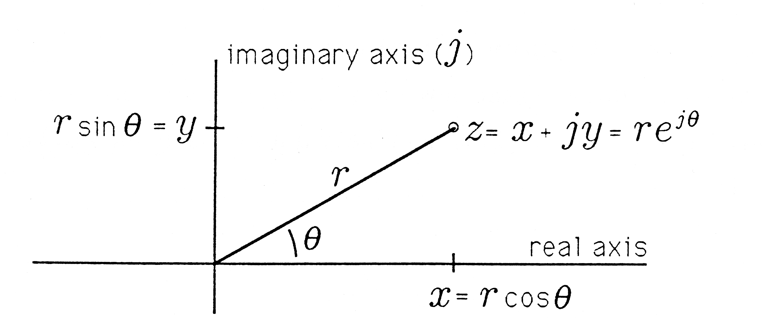
To solve this problem, we can begin by converting the point P from rectangular coordinates to polar coordinates. We have

(5.1)

The rotated point P ' has the same radius r , and its angle is . We now convert back to rectangular coordinates to find x ' and y ' for point P ' :

(5.2)

So the rotated point P ' has coordinates (2.10, 2.37).

Now imagine trying to rotate the graphical image of some complex object like an airplane. You could try to rotate all 10,000 (or so) points in the same way as the single point was just rotated. However, a much easier way to rotate all the points together is provided by linear algebra. In fact, with a single linear algebraic operation we can rotate and scale an entire object and project it from three dimensions to two for display on a flat screen or sheet of paper.

In this chapter we study vector graphics, a linear algebraic method of storing and manipulating computer images. Vector graphics is especially suited to moving, rotating, and scaling (enlarging and reducing) images and objects within images. Cropping is often necessary too, although it is a little more difficult with vector graphics. Vector graphics also allows us to store objects in three dimensions and then view the objects from various locations in space by using projections.

In vector graphics, pictures are drawn from straight lines.^[9] A curve can be approximated as closely as desired by a series of short, straight lines. Clearly some pictures are better suited to representation by straight lines than are others. For example, we can achieve a fairly good representation of a building or an airplane in vector graphics, while a photograph of a forest would be extremely difficult to convert to straight lines. Many computer- aided design (CAD) programs use vector graphics to manipulate mechanical drawings.

When the time comes to actually display a vector graphics image, it may be necessary to alter the representation to match the display device. Personal computer display screens are divided into thousands of tiny rectangles called picture elements, or pixels. Each pixel is either off (black) or on (perhaps with variable intensity and/or color). With a CRT display, the electron beam scans the rows of pixels in a raster pattern. To draw a line on a pixel display device, we must first convert the line into a list of pixels to be illuminated. Dot matrix and laser printers are also pixel display devices, while pen plotters and a few specialized CRT devices can display vector graphics directly. We will let MATLAB do the conversion to pixels and automatically handle cropping when necessary.

We begin our study of vector graphics by representing each point in an image by a vector. These vectors are arranged side-by-side into a matrix G containing all the points in the image. Other matrices will be used as operators to perform the desired transformations on the image points. For example, we will find a matrix R , which functions as a rotation: the matrix product RG represents a rotated version of the original image G .

Point Matrix. To represent a straight-line image in computer memory, we must store a list of all the endpoints of the line segments that comprise the image. If the point is such an endpoint, we write it as the column vector

(5.3)

Suppose there are n such endpoints in the entire image. Each point is included only once, even if several lines end at the same point. We can arrange the vectors P_i into a point matrix:

(5.4)

We then store the point matrix G∈R^2xn as a two-dimensional array in computer memory.

Example 5.2. 

Consider the list of points

(5.5)

The corresponding point matrix is

(5.6)

Line Matrix. The next thing we need to know is which pairs of points to connect with lines. To store this information for m lines, we will use a line matrix, H∈R^2×m. The line matrix does not store line locations directly. Rather, it contains references to the points stored in G . To indicate a line between points p_i and p_j, we store the indices i and j as a pair. For the k^th line in the image, we have the pair

(5.7)

The order of i and j does not really matter since a line from p_i to p_j is the same as a line from p_j to p_i. Next we collect all the lines h_k into a line matrix H :

(5.8)

All the numbers in the line matrix H will be positive integers since they point to columns of G . To find the actual endpoints of a line, we look at columns i and j of the point matrix G .

Example 5.3. 

To specify line segments connecting the four points of Example 1 into a quadrilateral, we use the line matrix

(5.9)

Alternatively, we can specify line segments to form a triangle from the first three points plus a line from P₃ to P₄ :

(5.10)

Figure 1 shows the points G connected first by H₁ and then by H₂.

Figure 5.2. 

Two Sets of Lines

Demo 1 (MATLAB). Use your editor to enter the following MATLAB function file. Save it as vgraphl.m.

function vgraphl (points, lines);
% vgraphl (points, lines) plots the points as *'s and
% connects the points with specified lines. The points
% matrix should be 2xN, and the lines matrix should be 2xM.
% The field of view is preset to (-50,50) on both axes.
%
% Written by Richard T. Behrens, October 1989
%
m=length(lines);                    % find the number of
                                    % lines.
axis([-50 50 -50 50])               % set the axis scales
axis('square')
plot(points(1,:),points(2,:),'*')   % plot the points as *
hold on                             % keep the points...
for i=i:m                           % while plotting the
                                    % lines
    plot([points(1,lines(1,i)) points(1,lines(2,i))],..
        [points(2,lines(2,lines(1,i)) points(2,lines(2,i))],'-')
    
    end
    
    hold off

After you have saved the function file, run MATLAB and type the following to enter the point and line matrices. (We begin with the transposes of the matrices to make them easier to enter.)

>> G = [
    0.6052 -0.4728;
   -0.4366  3.5555;
   -2.6644  7.9629;
   -7.2541 10.7547;
  -12.5091 11.5633;
  -12.5895 15.1372;
   -6.5602 13.7536;
  -31.2815 -7.7994;
  -38.8314 -9.9874;
  -44.0593 -1.1537;
  -38.8314  2.5453;
  -39.4017  9.4594;
  -39.3192 15.0932;
  -45.9561 23.4158]

>> G = G'

>> H = [
   1   2;
   2   3;
   3   4;
   4   5;
   4   7;
   5   6;
   8   9;
   9   10;
   10  11;
   11  12;
   12  13;
   12  14]

>> H = H'

At this point you should use MATLAB's “save” command to save these matrices to a disk file. Type

>> save dippers

After you have saved the matrices, use the function VGRAPH1 to draw the image by typing

≫ vgraph1(G,H)

The advantage of storing points and lines separately is that an object can be moved and scaled by operating only on the point matrix G . The line information in H remains the same since the same pairs of points are connected no matter where we put the points themselves.

Surfaces and Objects. To describe a surface in three dimensions is a fairly complex task, especially if the surface is curved. For this reason, we will be satisfied with points and lines, sometimes visualizing flat surfaces based on the lines. On the other hand, it is a fairly simple matter to group the points and lines into distinct objects. We can define an object matrix K with one column for each object giving the ranges of points and lines associated with that object. Each column is defined as

(5.11)

As with the line matrix H , the elements of K are integers.

Example 5.4. 

Consider again Demo 1. We could group the points in G and the lines in H into two objects with the matrix

(5.12)

The first column of K specifies that the first object (Ursa Minor) is made up of points 1 through 7 and lines 1 through 6, and the second column of K defines the second object (Ursa Major) as points 8 through 14 and lines 7 through 12.

We now turn our attention to operating on the point matrix G to produce the desired transformations. We will consider rotation; scaling; and translation (moving) of objects. Rotation and scaling are done by matrix multiplication with a square transformation matrix A. If we call the transformed point matrix G_new, we have

(5.13)

We call A a matrix operator because it “operates” on G through matrix multiplication. In contrast, translation must be done by matrix addition.

In a later section you will see that it is advantageous to perform all operations by matrix operators and that we can modify our image representation to allow translation to be done with a matrix operator like rotation and scaling. We will call the modified representation homogeneous coordinates.

Rotation. We saw in the chapter on linear algebra that the matrix that rotates points by an angle θ is

(5.14)

When applied to the point matrix G, this matrix operator rotates each point by the angle θ, regardless of the number of points.

Example 5.5. 

We can use the rotation matrix to do the single point rotation of the example from "Vector Graphics: Introduction". We have a point matrix consisting of only the point (3,1):

(5.15)

The necessary transformation matrix is R(θ) with Then the rotated point is given by

(5.16)

Scaling. An object can be enlarged or reduced in each dimension inde- pendently. The matrix operator that scales an image by a factor of s_x along the x-axis and s_y along the y-axis is

(5.17)

Most often we take s_x=s_y to scale an image by the same amount in both dimensions.