This module is part of the collection, A First Course in Electrical and Computer Engineering. The LaTeX source files for this collection were created using an optical character recognition technology, and because of this process there may be more errors than usual. Please contact us if you discover any errors.
When we teach complex numbers to beginning engineering students, we encourage a geometrical picture supported by an algebraic structure. Every algebraic manipulation carried out in a lecture is accompanied by a care-fully drawn picture in order to fix the idea that geometry and algebra go hand-in-glove to complete our understanding of complex numbers. We assign essentially every problem for homework.
We use the MATLAB programs in this chapter to illustrate the theory of complex numbers and to develop skill with the MATLAB language. The numerical experiment introduces students to the basic quadratic equation of electrical and computer engineering and shows how the roots of this quadratic equation depend on the coefficients of the equation.
“Representing Complex Numbers in a Vector Space,” is a little demanding for freshmen but easily accessible to sophomores. It may be covered for additional insight, skipped without consequence, or covered after Chapter 4. “An Electric Field Computation,” is well beyond most freshmen, and it is demanding for sophomores. Nonetheless, an expert in electromagnetics might want to cover the section "An electric Field Computation" for the insight it brings to the use of complex numbers for representing two-dimensional real quantities.
It is hard to overestimate the value of complex numbers. They first arose in the study of roots for quadratic equations. But, as with so many other great discoveries, complex numbers have found widespread application well outside their original domain of discovery. They are now used throughout mathematics, applied science, and engineering to represent the harmonic nature of vibrating systems and oscillating fields. For example, complex numbers may be used to study
traveling waves on a sea surface;
standing waves on a violin string;
the pure tone of a Kurzweil piano;
the acoustic field in a concert hall;
the light of a He-Ne laser;
the electromagnetic field in a light show;
the vibrations in a robot arm;
the oscillations of a suspension system;
the carrier signal used to transmit AM or FM radio;
the carrier signal used to transmit digital data over telephone lines; and
the 60 Hz signal used to deliver power to a home.
In this chapter we develop the algebra and geometry of complex numbers. In Chapter 3 we will show how complex numbers are used to build phasor representations of power and communication signals.
This module is part of the collection, A First Course in Electrical and Computer Engineering. The LaTeX source files for this collection were created using an optical character recognition technology, and because of this process there may be more errors than usual. Please contact us if you discover any errors.
The most fundamental new idea in the study of complex numbers is the “imaginary number” j. This imaginary number is defined to be the square root of – 1 :

The imaginary number j is used to build complex numbers x and y in the following way:
We say that the complex number z has “real part” x and “imaginary part” y:

In MATLAB, the variable x is denoted by real(z), and the variable y is
denoted by imag(z). In communication theory, x is called the “in-phase”
component of z, and y is called the “quadrature” component. We call z=x+jy the Cartesian representation of z, with real component x and imaginary component y. We say that the Cartesian pair (x,y)codes the complex
number z.
We may plot the complex number z on the plane as in Figure 1.1. We call the horizontal axis the “real axis” and the vertical axis the “imaginary axis.” The plane is called the “complex plane.” The radius and angle of the line to the point z=x+jy are


See Figure 1.1. In MATLAB, r is denoted by abs(z), and θ is denoted by angle(z).
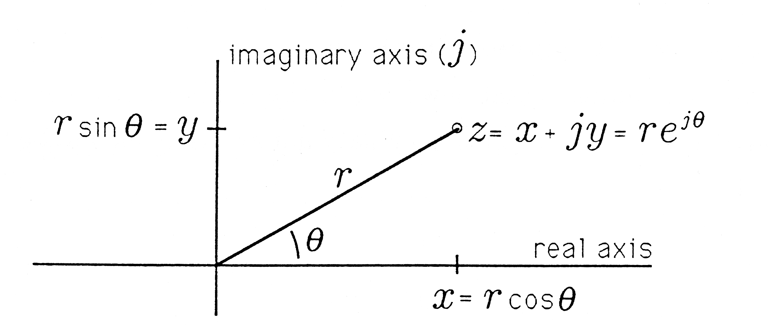
The original Cartesian representation is obtained from the radius r and angle θ as follows:

The complex number z may therefore be written as

The complex number cosθ+jsinθ is, itself, a number that may be represented on the complex plane and coded with the Cartesian pair (cosθ,sin θ) . This is illustrated in Figure 1.2. The radius and angle to the point z=cosθ+jsin θ are 1 and θ. Can you see why?
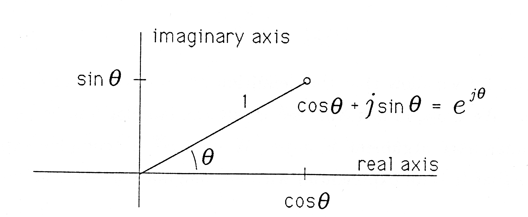

The complex number cosθ+jsinθ is of such fundamental importance to our study of complex numbers that we give it the special symbol ejθ :
As illustrated in Figure 1.2, the complex number ejθ has radius 1 and angle θ. With the symbol ejθ, we may write the complex number z as
We call z=rejθ a polar representation for the complex number z. We say that the polar pair r∠θcodes the complex number z. In this polar representation, we define |z|=r to be the magnitude of z and arg(z)=θ to be the angle, or phase, of z:

With these definitions of magnitude and phase, we can write the complex number z as
Let's summarize our ways of writing the complex number z and record the corresponding geometric codes:

In "Roots of Quadratic Equations" we show that the definition ejθ=cosθ+jsinθ is more than symbolic. We show, in fact, that ejθ is just the familiar function ex evaluated at the imaginary argument x=jθ. We call ejθ a “complex exponential,” meaning that it is an exponential with an imaginary argument.
Prove (j)2n=(–1)n and (j)2n+1=(–1)nj. Evaluate j3,j4,j5.
Prove ej[(π/2)+m2π]=j,ej[(3π/2)+m2π]=–j,ej(0+m2π)=1, and ej(π+m2π)=–1. Plot these identities on the complex plane. (Assume m is an integer.)
Find the polar representation z=rejθ for each of the following complex numbers:
z=1+j0;
z=0+j1;
z=1+j1;
z=–1–j1.
Plot the points on the complex plane.
Find the Cartesian representation z=x+jy for each of the following complex numbers:
 ;
;
 ;
;
z=ej3π/4 ;
 .
.
Plot the points on the complex plane.
The following geometric codes represent complex numbers. Decode each by writing down the corresponding complex number z:
 ?
?
 ?
?
 ?
?
 ?
?
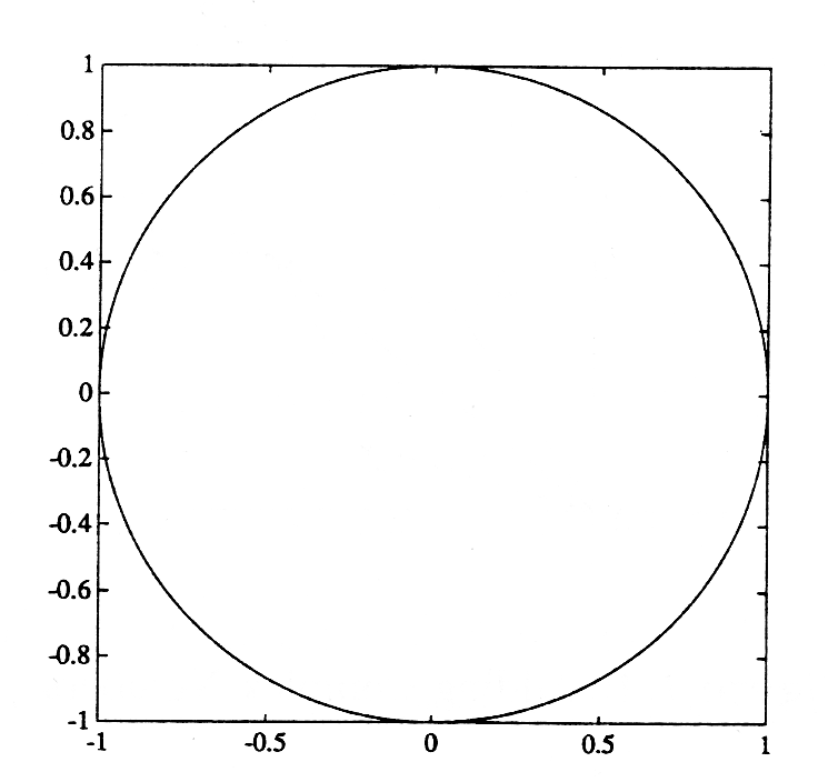
Show that Im[jz]= Re [z] and Re [–jz]= Im [z]. Demo 1.1 (MATLAB). Run the following MATLAB program in order to compute and plot the complex number ejθ for θ=i2π/360,i=1,2,...,360:
          j=sqrt(-1)
          n=360
          for i=1:n,circle(i)=exp(j*2*pi*i/n);end;
          axis('square')
          plot(circle)
Replace the explicit for loop of line 3 by the implicit loop
circle=exp(j*2*pi*[1:n]/n);
to speed up the calculation. You can see from Figure 1.3 that the complex number ejθ, evaluated at angles θ=2π/360,2(2π/360),..., turns out complex numbers that lie at angle θ and radius 1. We say that ejθ is a complex number that lies on the unit circle. We will have much more to say about the unit circle in Chapter 2.