This module is part of the collection, A First Course in Electrical and Computer Engineering. The LaTeX source files for this collection were created using an optical character recognition technology, and because of this process there may be more errors than usual. Please contact us if you discover any errors.
It is essential to write out, term-by-term, every sequence and sum in this chapter. This demystifies the seemingly mysterious notation. The example on compound interest shows the value of limiting arguments in everyday life and gives ex some real meaning. The function ejθ, covered in the section "The Function of ejθ and the Unit Circle and "Numerical Experiment (Approximating ejθ, must be understood by all students before proceeding to "Phasors" . The Euler and De Moivre identities provide every tool that students need to derive trigonometric formulas. The properties of roots of unity are invaluable for the study of phasors in "Phasors" .
The MATLAB programs in this chapter are used to illustrate sequences and series and to explore approximations to sin θ and cos θ . The numerical experiment in "Numerical Experiment (Approximating ejθ illustrates, geometrically and algebraically, how approximations to ejθ converge.
“Second-Order Differential and Difference Equations” is a little demanding for freshmen, but we give it a once-over-lightly to illustrate the power of quadratic equations and the functions ex and ejθ. This section also gives a sneak preview of more advanced courses in circuits and systems.
It is probably not too strong a statement to say that the function ex is the most important function in engineering and applied science. In this chapter we study the function ex and extend its definition to the function ejθ. This study clarifies our definition of ejθ from "Complex Numbers" and leads us to an investigation of sequences and series. We use the function ejθ to derive the Euler and De Moivre identities and to produce a number of important trigonometric identities. We define the complex roots of unity and study their partial sums. The results of this chapter will be used in "Phasors" when we study the phasor representation of sinusoidal signals.
This module is part of the collection, A First Course in Electrical and Computer Engineering. The LaTeX source files for this collection were created using an optical character recognition technology, and because of this process there may be more errors than usual. Please contact us if you discover any errors.
Many of you know the number e as the base of the natural logarithm, which has the value 2.718281828459045. . . . What you may not know is that this number is actually defined as the limit of a sequence of approximating numbers. That is,


This means, simply, that the sequence of numbers  ,
. . . , gets arbitrarily close to 2.718281828459045. . . . But why should such
a sequence of numbers be so important? In the next several paragraphs we
answer this question.
,
. . . , gets arbitrarily close to 2.718281828459045. . . . But why should such
a sequence of numbers be so important? In the next several paragraphs we
answer this question.
(MATLAB) Write a MATLAB program to evaluate the expression  for n=1,2,4,8,16,32,64 to show that fn≈e for large
n.
for n=1,2,4,8,16,32,64 to show that fn≈e for large
n.
Derivatives and the Number e. The number  arises
in the study of derivatives in the following way. Consider the function
arises
in the study of derivatives in the following way. Consider the function

and ask yourself when the derivative of f(x) equals f(x). The function f(x) is plotted in Figure 2.1 for a>1. The slope of the function at point x is

If there is a special value for a such that

then  would equal f(x). We call this value of a the special (or exceptional) number e and write

The number e would then be e=f(1). Let's write our condition that  converges to 1 as

or as
Our definition of  amounts to defining
  and
allowing n→∞ in order to make Δx→0. With this definition for e, it is
clear that the function
ex is defined to be (e)x :
and
allowing n→∞ in order to make Δx→0. With this definition for e, it is
clear that the function
ex is defined to be (e)x :

By letting  we can write this definition in the more familiar form

This is our fundamental definition for the function ex. When evaluated at x=1, it produces the definition of e given in Equation 2.1.
The derivative of ex is, of course,

This means that Taylor's theorem[3] may be used to find another characterization for ex :

When this series expansion for ex is evaluated at x=1, it produces the following series for e:

In this formula, n! is the product n(n–1)(n–2)⋯( 2 ) 1 . Read n! as " n factorial.”
(MATLAB) Write a MATLAB program to evaluate the sum

for N=1,2,4,8,16,32,64 to show that SN≅e for large N . Compare S64 with f64 from Exercise 1.. Which approximation do you prefer?
Compound Interest and the Function  . There is an example
from your everyday life that shows even more dramatically how the function
ex
arises. Suppose you invest
V0 dollars in a savings account that offers
100
x
%
annual interest. (When x=0.01, this is 1%; when x=0.10, this is 10%
interest.) If interest is compounded only once per year, you have the simple interest formula for
V1, the value of your savings account after 1 compound
(in this case, 1 year):
. There is an example
from your everyday life that shows even more dramatically how the function
ex
arises. Suppose you invest
V0 dollars in a savings account that offers
100
x
%
annual interest. (When x=0.01, this is 1%; when x=0.10, this is 10%
interest.) If interest is compounded only once per year, you have the simple interest formula for
V1, the value of your savings account after 1 compound
(in this case, 1 year):
V1=(1+x)V0. This result is illustrated in the block diagram of Figure 2.2(a). In this diagram, your input fortune V0 is processed by the “interest block” to produce your output fortune V1. If interest is compounded monthly, then the annual interest is divided into 12 equal parts and applied 12 times. The compounding formula for V12, the value of your savings after 12 compounds (also 1 year) is

This result is illustrated in Figure 2.2b. Can you read the block diagram? The general formula for the value of an account that is compounded n times per year is

Vn is the value of your account after n compounds in a year, when the annual interest rate is 100x%.
Verify in Equation 2.16 that a recursion is at work that terminates at
Vn. That is, show that
 for i=0,1,...,n–1
produces the result
for i=0,1,...,n–1
produces the result  .
.
Bankers have discovered the (apparent) appeal of infinite, or continuous, compounding:

We know that this is just
So, when deciding between 100x1 % interest compounded daily and 100x2% interest compounded continuously, we need only compare

We suggest that daily compounding is about as good as continuous compounding. What do you think? How about monthly compounding?
(MATLAB) Write a MATLAB program to compute and plot simple interest, monthly interest, daily interest, and continuous interest versus interest rate 100x. Use the curves to develop a strategy for saving money.
This module is part of the collection, A First Course in Electrical and Computer Engineering. The LaTeX source files for this collection were created using an optical character recognition technology, and because of this process there may be more errors than usual. Please contact us if you discover any errors.
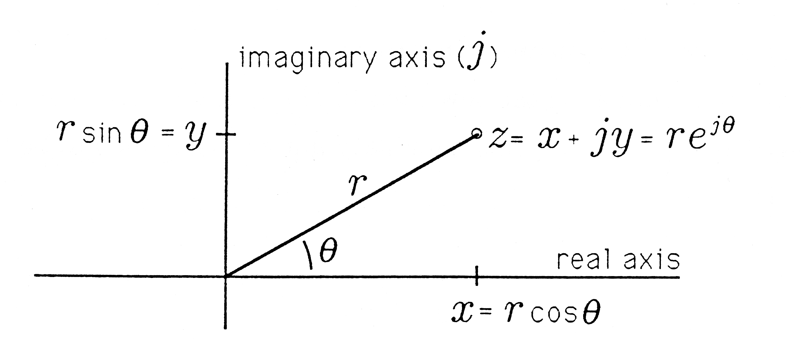
Let's try to extend our definitions of the function ex to the argument x = j Θ . Then ejΘ is the function
The complex number  is illustrated in Figure 2.3. The radius to the
point
is illustrated in Figure 2.3. The radius to the
point  is
is  and the angle is
  This means that
the nth power of has radius
This means that
the nth power of has radius  and angle
  (Recall our study of powers of z.) Therefore the complex number
  may be written as

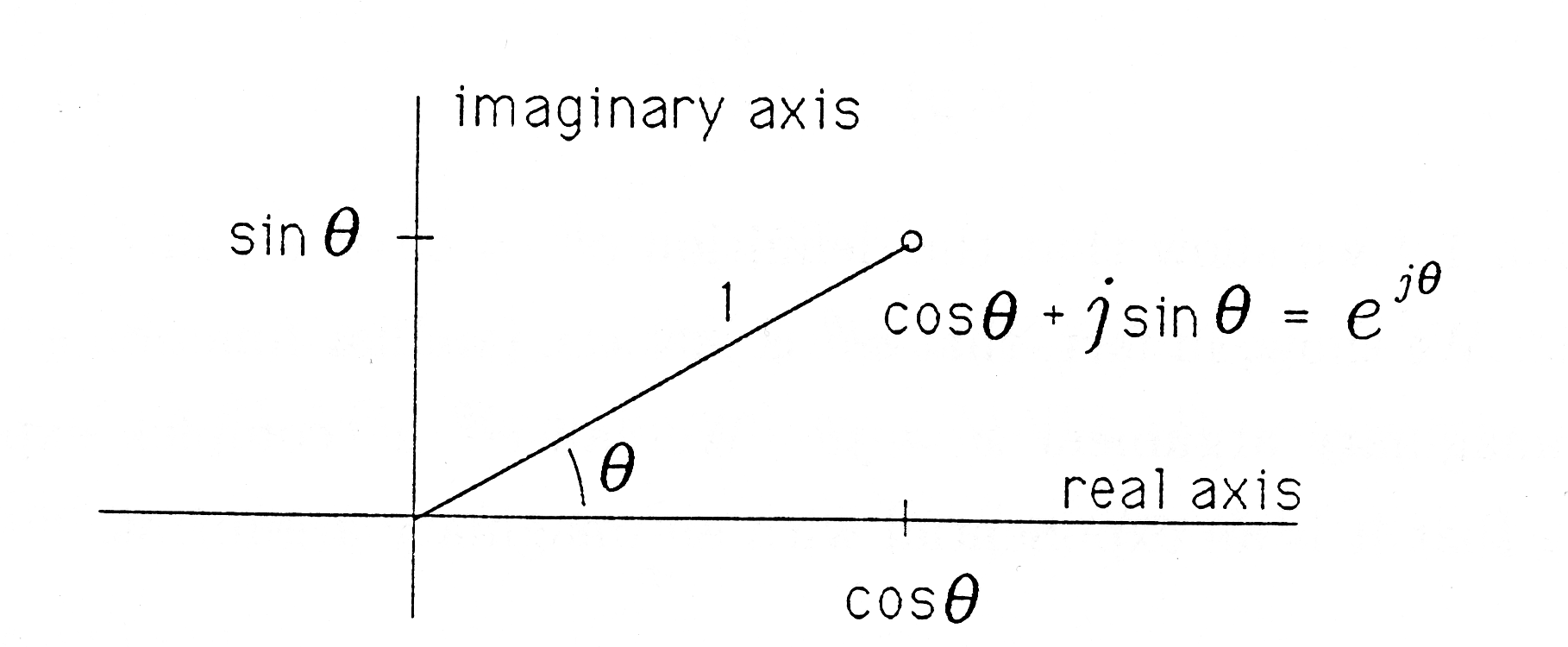
For n large,  , and . Therefore
is approximately
, and . Therefore
is approximately

 ( cosθ+j sin θ).
This finding is consistent with our previous definition of