Beam Element - A beam element is a slender structural member that offers resistance to forces and bending under applied loads. A beam element differs from a truss element in that a beam resists moments (twisting and bending) at the connections.
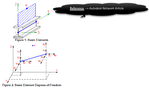
These three node elements are formulated in three-dimensional space. The first two nodes (I-node and J-node) are specified by the element geometry. The third node (K-node) is used to orient each beam element in 3-D space (see Figure 1). A maximum of three translational degrees-of-freedom and three rotational degrees-of-freedom are defined for beam elements (see Figure 2). Three orthogonal forces (one axial and two shear) and three orthogonal moments (one torsion and two bending) are calculated at each end of each element. Optionally, the maximum normal stresses produced by combined axial and bending loads are calculated. Uniform inertia loads in three directions, fixed-end forces, and intermediate loads are the basic element based loadings.
The basic guidelines for when to use a beam element are:
Solid Element – Solid elements are three-dimensional finite elements that can model solid bodies and structures without any a priori geometric simplification.
Finite element models of this type have the advantage of directness. Geometric, constitutive and loading assumptions required to effect dimensionality reduction, for example to planar or axisymmetric behavior, are avoided. Boundary conditions on both forces and displacements can be more realistically treated. Another attractive feature is that the finite element mesh visually looks like the physical system.
Summarizing, use of solid elements should be restricted to problem and analysis stages, such as verification, where the generality and flexibility of full 3D models is warranted. They should be avoided during design stages. Furthermore they should also be avoided in thin-wall structures such as aerospace shells, since solid elements tend to perform poorly because of locking problems.
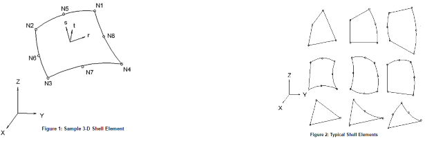
Shell Element – Shell elements are 4- to 8-node isoparametric quadrilaterals or 3- to 6-node triangular elements in any 3-D orientation. The 4-node elements require a much finer mesh than the 8-node elements to give convergent displacements and stresses in models involving out-of-plane bending. Figure 1 shows some typical shell elements.
The General and Co-rotational shell element is formulated based on works by Ahmad, Iron and Zienkiewicz and later refined by Bathe and Balourchi. It can be applied to model both thick and thin shell problems. Also, the geometry of a doubly curved shell with variable thickness can be accurately described using this shell element.
The Thin shell element is based on thin plate theory. The bending behavior of the element is based on a discrete Kirchhoff approach to plate bending using Batoz's interpolation functions. This formulation satisfies the Kirchhoff constraints along the boundary and provides linear variation of curvature through the element. The membrane behavior of the element is based on the Allman triangle which is derived from the Linear Strain Triangular (LST) element. A general curved surface is approximated by this element as a set of facets formed by the planes defined by the three nodes of each element. For these reason a well-refined mesh is necessary.
The element geometry is described by the nodal point coordinates. Each shell element node has 5 degrees of freedom (DOF) - three translations and two rotations. The translational DOF are in the global Cartesian coordinate system. The rotations are about two orthogonal axes on the shell surface defined at each node. The rotational boundary condition restraints and applied moments also refer to this nodal rotational system. The two rotational axes (V1 and V2) are usually automatically determined by the processor and you do not have to specifically orient them.
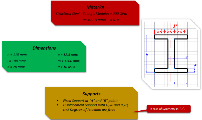
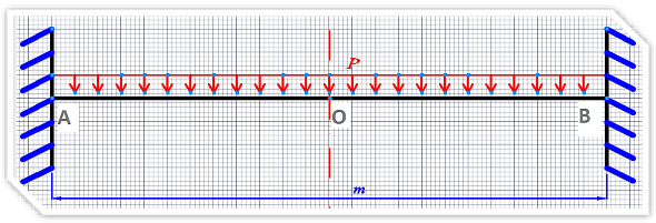
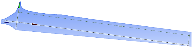
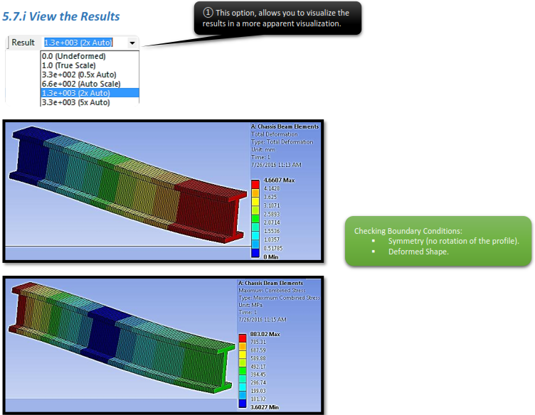
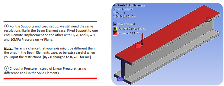
To be able to make the comparison between beam, solid and surface elements we are going to need a geometry which is compatible with all 3 parameters. That is why we are going to use a part of a Car Chassis with dimensions and loads which are given below.
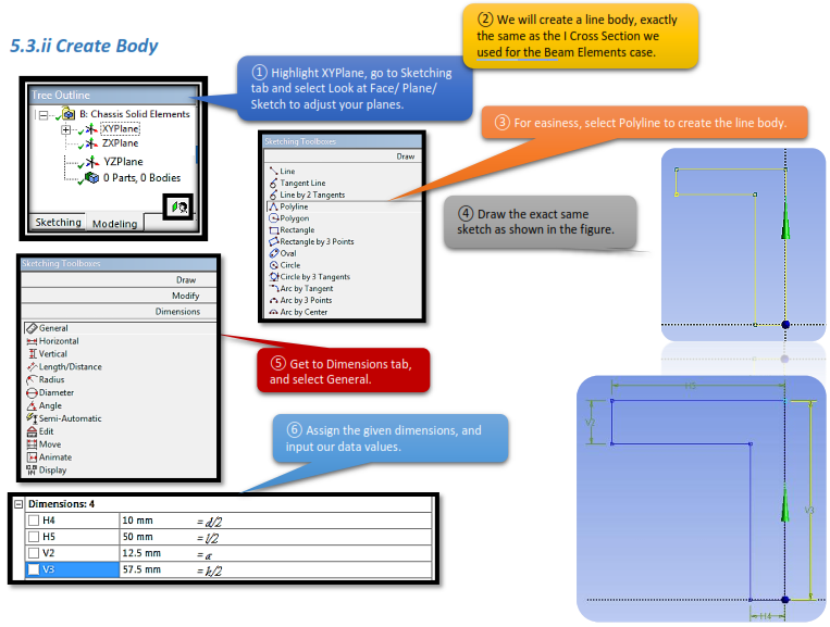
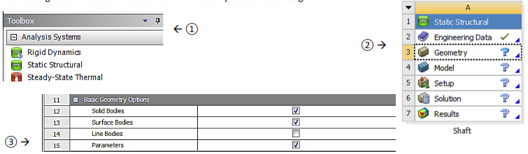
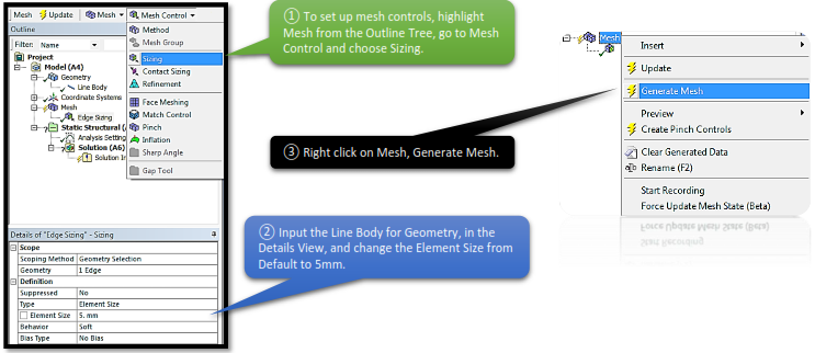
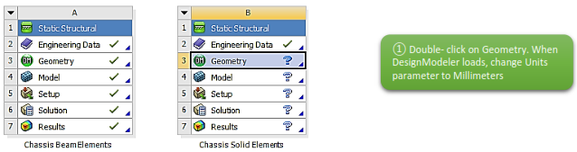
Once you opened up ANSYS Workbench, create a new Static Structural System and save your study case to a proper destination folder. Afterwards open the Engineering Data tab and make sure that the material properties match our data. Getting back now to the Project tab, we need to make an adjustment, since we are working with Beam Elements. For that reason, highlight Geometry from the Static Structural System and tick the box in the Basic Geometry Options tab, the once concerning the Line Bodies. Double click on Geometry to start sketching.
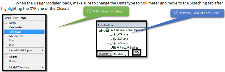
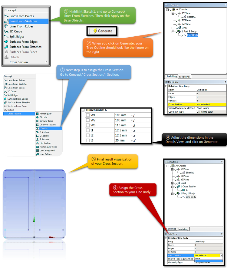
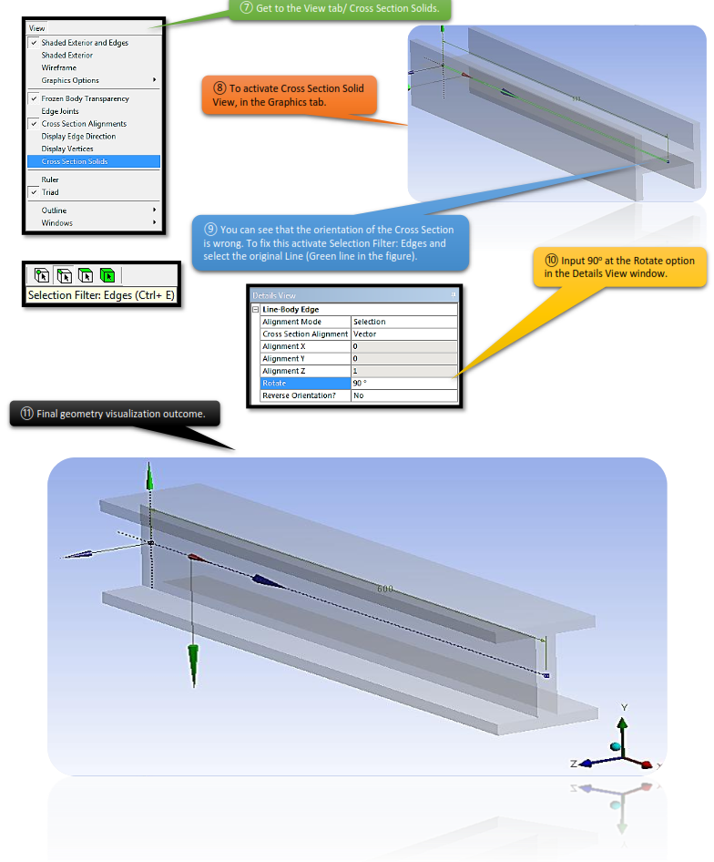
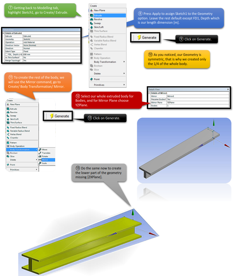
As you noticed in the Problem Description paragraph, our model is symmetric, meaning that we got the option here to sketch only half of the geometries body without having differences at the end results. So, getting back to the sketching part, we will need firstly to create just a single line and then it’s Cross-Section.
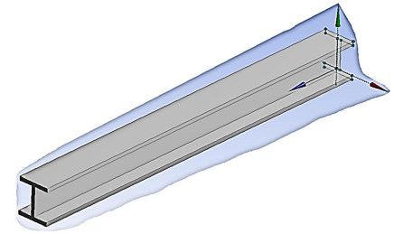
Your Geometry Body is ready, close DesignModeler and open up Mechanical GUI, by double clicking on the Model from the Static Structural System (we do not need to make any modifications in this case before opening up Mechanical GUI).
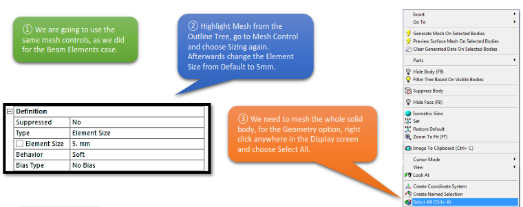
Next part of this chapter would be, creating the same geometry, with the same boundary conditions, the same loads. Only difference would be that, this time we will use solid elements for our analysis. Open up your previous study case (Car Chassis), and create a new Static Structural System, check again your Engineering Data to much with our data and leave everything else as default· open up DesignModeler, and change your Units to Millimeters.
After finishing with sketching the geometry, close DesignModeler and open up Mechanical GUI, by double clicking on the Model from the Static Structural System (there is no need to make any modifications).
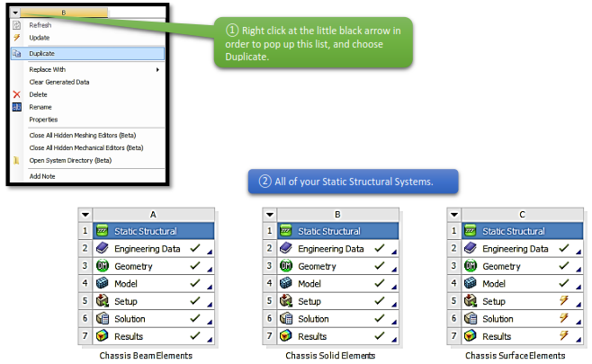
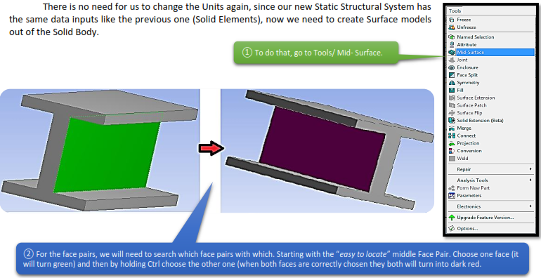
In this study case, it will not be needed to create a new Static Structural System and sketching the geometry from all over again. There is an easier way by Duplicating the Solid Elements study case, with this option the newly created Static Structural System has the exact same geometry, mesh and boundary conditions like the Static Structural System that we Duplicated. After Duplicating it, open up DesignModeler to make some modifications regarding the Surface Elements.
One of the better features of Workbench’s DesignModeler is the Mid-Surface Extraction tool. This tool is fairly simple to use, and after some practice, you will be creating shell models in no time. The Mid-Surface Extraction utility is located underneath the ‘Tools’ Menu.
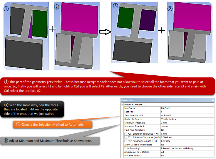
The easiest way to create Mid-Surfaces is to manually go through and select the face pairs. You will notice that after selecting the “top” and “bottom” face, they will appear as two different colors. It is important to note that the order in which you click the two faces determines the ”top” and ”bottom” of the shell element (important for applying pressures/defining contact). The shell normal is positive going from the pink (2nd pick) to the purple (1st pick) surface.
You can select multiple face pairs, then go back and hit the apply button for “Face Pairs” in the detail window. If there are several face pairs that have the same thickness, you can select one pair, then go back and change the selection type to be automatic. This will fill in some blanks in the details window.
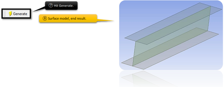
Finally, change “Find Face Pairs Now” to be “Yes” and DesignModeler will go out and find all face pairs that meet this criteria. Hit generate and all of your midplanes will be generated, and all thicknesses will be stored for later use in Simulation.
We are done with the DesignModeler, so feel free to close the window, and open Mechanical GUI by double clicking at the Model from the Static Structural System. A pop up window will appear asking you if you want to read the up-stream data, which means that the Mechanical GUI will automatically load the new changes we made in the DesignModeler, click Yes.
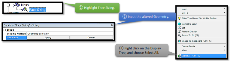
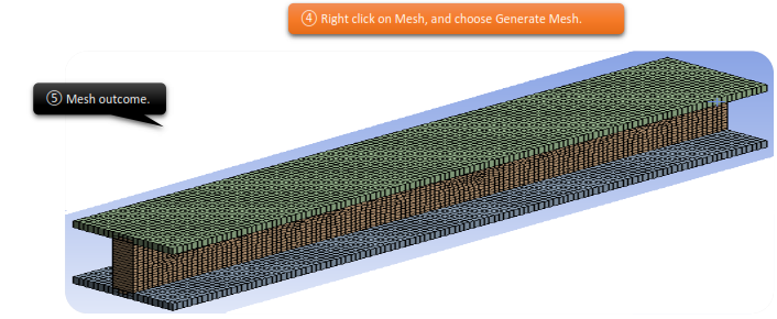
As you probably already understood, we are not going to change the mesh, the supports, the loads or the solution outcomes. Thanks to the Duplication the parameters are already settled and we just need to define the new changed geometry.
iv. Type of Elements Comparison
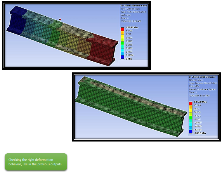
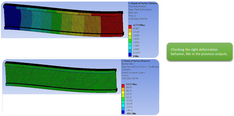
We could compare and comment the results of all 3 different type of elemets.