A structure of revolution by itself does not necessarily define an axisymmetric problem. It is also necessary that the loading, as well as the support boundary conditions, be rotationally symmetric.
Axisymmetric elements are 2D elements that can be used to model axisymmetric geometries with axisymmetric load. In simpler words, we are converting a 3D Geometry to a 2D Geometry making the model smaller, therefore faster execution and faster post processing.
We only model the cross section, and ANSYS accounts for the fact that it is really a 3D, axisymmetric structure.
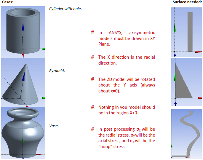
Examples before beginning our task
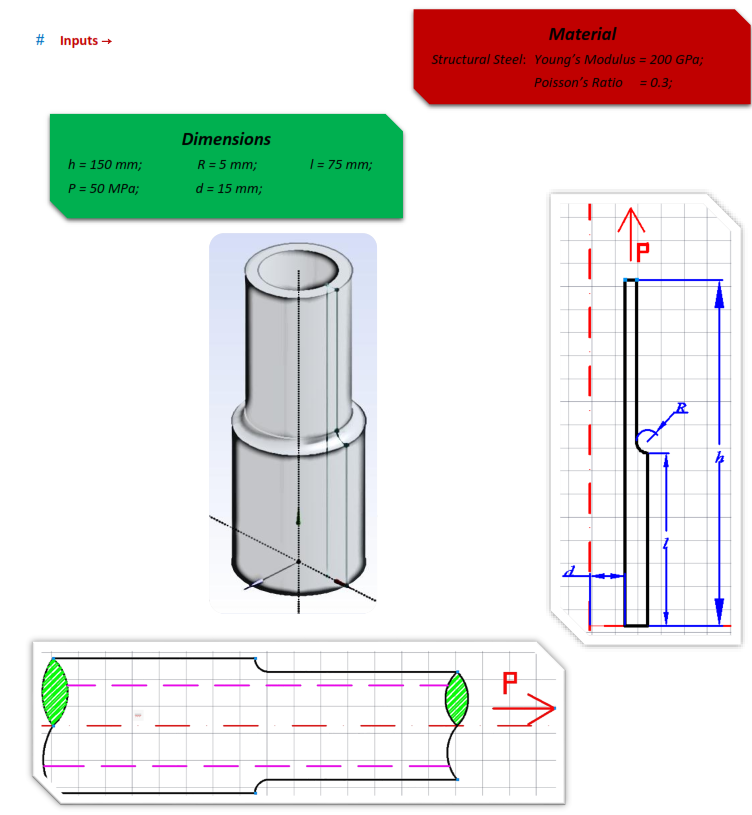
In this chapter we consider the finite element discretization of axisymmetric solids. We were given a Steel Shaft with dimensions which are given below. Purpose of this chapter is to evaluate stress concentration factor of the shaft notch, compare the result with the experimental data and fully understand the concept of Axi-symmetry and its possibilities.
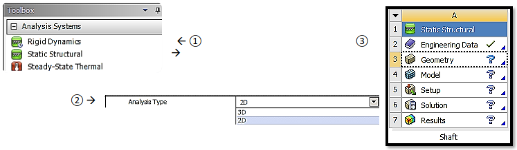
Open ANSYS Workbench, create a Static Structural system, and make sure that you saved your case study before moving forward. Next step is opening Engineering Data tab, to check if the material properties are correct. After doing, that highlight Geometry and change the Analysis Type on your right, from 3D to 2D. Double-click Geometry to start sketching.
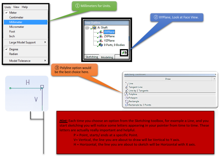
 After DesignModeler opens, get to the Units tab, and select Millimeter. Highlight XYPlane and start sketching.
4.3.1 Getting back to the Modeling
After finishing your sketch, close DesignModeler and open up Mechanical. First thing we need to adjust before start dealing with the Analysis, is to change Geometry’s behavior.
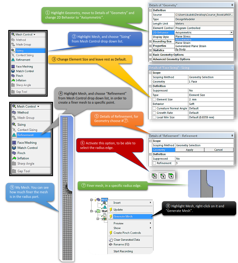
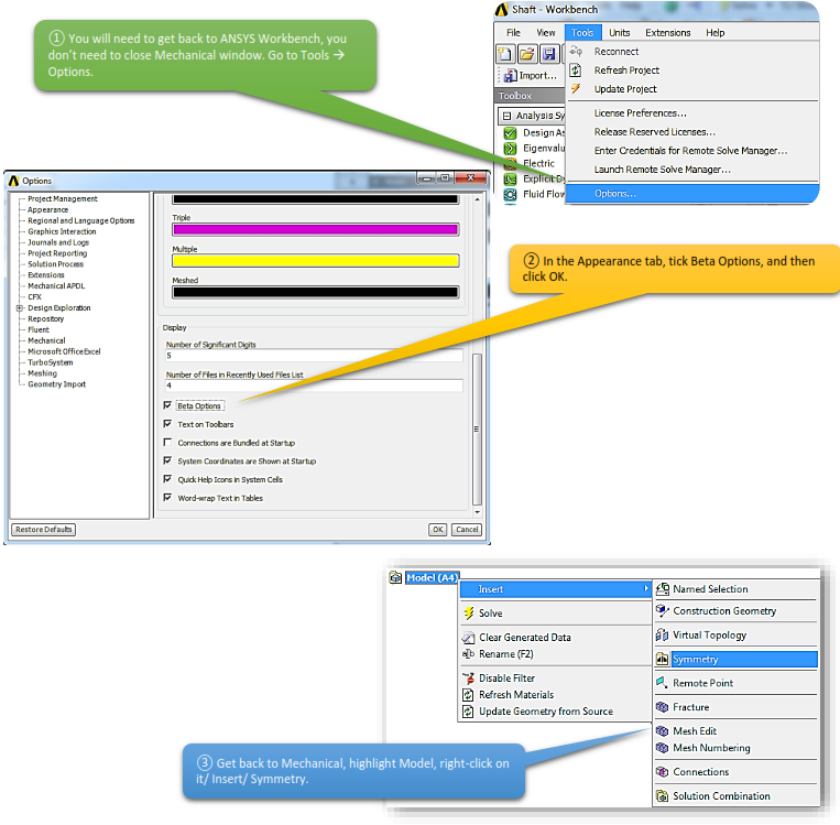
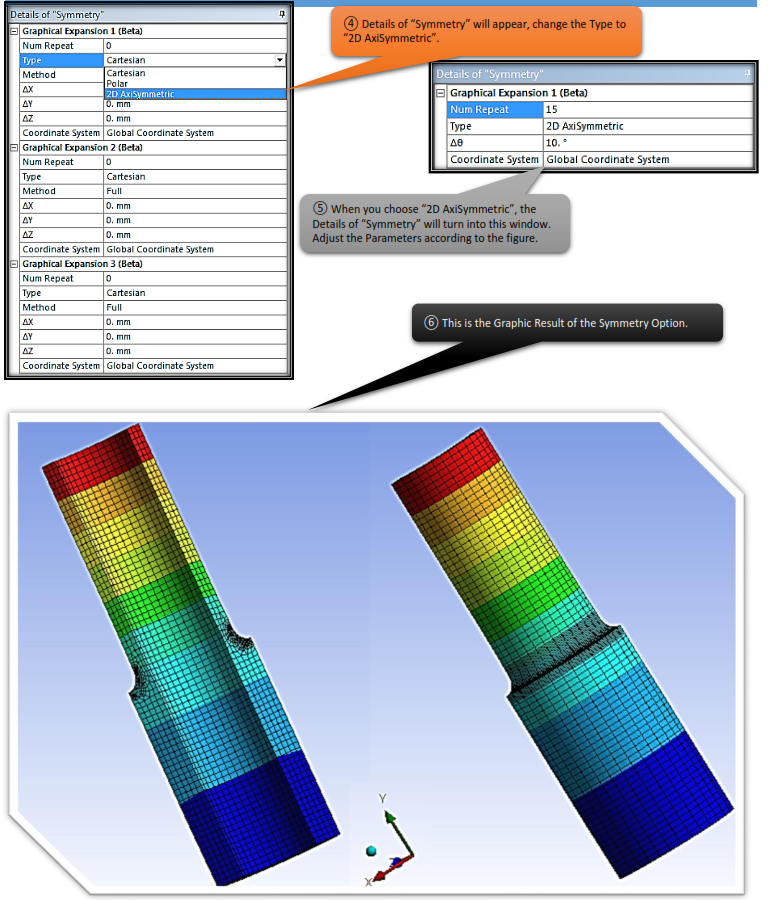
To help you understand the ideology of Axisymmetry, I will have to show you how to activate a couple of options to make a better visualization output of the results.
A stress concentration is a location in an object where stress is concentrated. An object is strongest when force is evenly distributed over its area, so a reduction in area, e.g. caused by a crack, results in a localized increase in stress. A material fail, via a propagating crack, when a concentrated stress exceeds the material’s theoretical cohesive strength. The real fracture strength of a material is always lower than the theoretical value because most materials contain small cracks or contaminants that concentrate stress.
The stress concentrators are geometrical irregularities that cause an increase in the average effort that should be present in regions near these discontinuities, the relationship between the maximum stress that occurs and the average effort that should occur is defined as stress concentration factor; which is determined by experimental or analytical methods and presented in graphical form for ease interpretation.
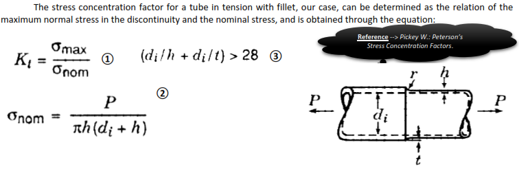
The stress concentration factor for a tube in tension with fillet, our case, can be determined as the relation of the maximum normal stress in the discontinuity and the nominal stress, and is obtained through the equation:
4.9.1 Hand Calculations VS Computational Calculations of Stress Concentration
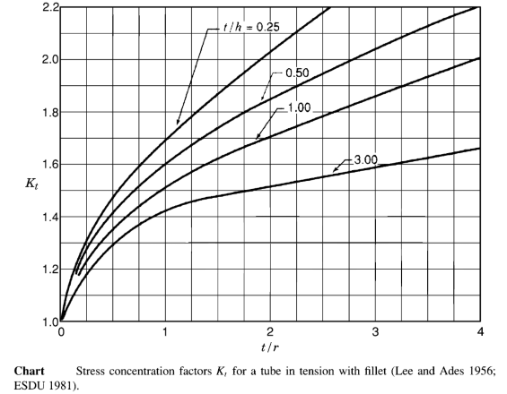
As we can see in the graph, there are 2 parameters that are taken into consideration to acquire stress concentration factor. First parameter would be to determine which line we need to choose, to accomplish that we have to solve the equation t/h with our given values. Second parameter would be to acquire the correct output for the X axis, solving the equation t/r.
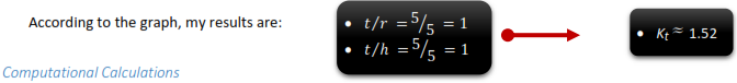
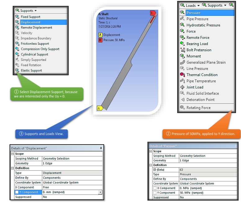
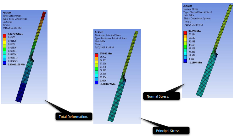
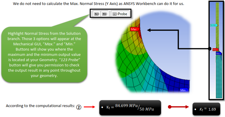
To acquire the Stress Concentration Factor for the computational calculations we are going to need Max. Normal Stress (Y Axis) and Nominal Stress, which in our case equals to 50MPa because of Pressure.

Conclusion: As we can see the results between Hand and Computational Calculations are almost the same. The difference of 11% is probably because of the geometry. Geometry proportion does not meet the criterion for the experimental data in the Stress Concentration Factor diagram, [Eq.  ]. The Geometry proportion coefficient should be greater than 28.
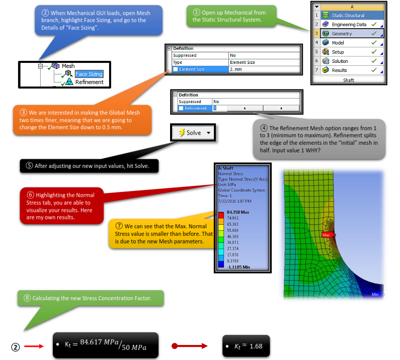
At this point we come across with an opportunity, to help you understand the concepts and the possibilities of Mesh and its options. To be more specific, we will change our element and node parameters (make it smaller, and finer), to check what happens to the Stress Concentration Factor. We are aiming to reduce the difference to a minimum value.
We can see that, we may got a difference in the Stress Concentration Factor but it is negligible.