4.5. Analyses of Circuit Simulations*
Analysis of Circuit Simulation
Multisim offers many analyses, all of which utilize simulation to generate the data for the desired analysis. These analyses range from quite basic to extremely sophisticated, and often require one analysis to be performed as part of another. To configure and begin an analysis, select Simulate/Analyses, and choose the desired analysis. Figure 1 lists all available Multisim analyses.
For each analysis, you configure the settings that tell Multisim how to exactly perform the desired analysis. In addition to the analyses provided by Multisim, user-defined analyses can be created based on user-entered SPICE commands.
To prepare an analysis, configure the analysis-specific parameters, such as frequency range for an AC analysis. Output traces must also be selected here. It is especially important to name nets appropriately to avoid confusion when analyzing results. The results are displayed on a plot in Multisim’s Grapher and saved for use in the Postprocessor. Some results are also written to an audit trail, which can be viewed.
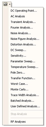
Figure 4.24.
Available Analyses
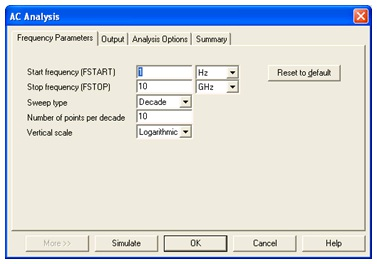
Figure 4.25.
AC Analysis Options Dialog Box
Grapher
The Grapher is the primary tool used to view the results of simulations. Users can view the Grapher by clicking View/Grapher. Additionally, the Grapher opens automatically displayed upon when running an analysis. Elements of the Grapher window are detailed in Figure 3.
The display shows both graphs and charts. In a graph, data are displayed as one or more traces along vertical and horizontal axes. In a chart, text data are displayed in rows and columns. The window is made up of several tabbed pages, depending on how many analyses, etc. have been run.
Each page has two possible active areas which will be indicated by a red arrow: the entire page indicated with the arrow in the left margin near the page name or the chart/graph indicated with the arrow in the left margin near the active chart/graph. Some functions, such as cut/copy/paste, affect only the active area, so be sure the desired area has been selected before performing a function.
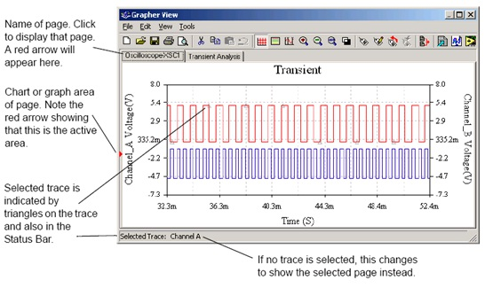
Figure 4.26.
The Grapher
Through the properties pages, the Grapher provides extensive customization. Axes scales, ranges, titles, colors, line styles, and many more options can be modified. To access the page or standard properties pages, click Edit/Page Propertiesor Edit/Properties (Figure 4 and Figure 5).
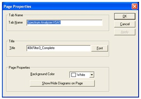
Figure 4.27.
Grapher Page Properties
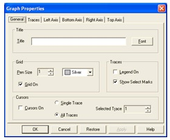
Figure 4.28.
Graph Properties
Cursors can be moved by clicking and dragging them with the mouse. Additionally, right-clicking on a cursor, will display cursor movement options. Users can move the cursor to a particular X-Value, Y-Value, and local Maxima or Minima in either direction (Figure 6). Cursors, legends and graph lines can be toggled on or off by clicking the corresponding toolbar buttons (Figure 7).
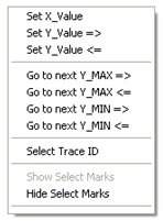
Figure 4.29.
Cursor Movement Options
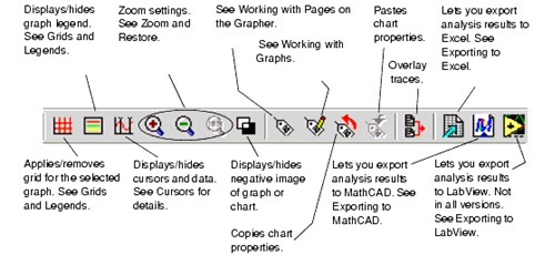
Figure 4.30.
Grapher Toolbar
Results can also be exported to NI LabVIEW, Excel, or MathCAD. Graph data can also be saved to a variety of formats including NI LabVIEW Data (either .LVM or .TDM), comma separated values (.CSV), and plain text. To save results from the Grapher select File/Save As,and choose the desired file format.