Introduction to Multisim Schematic Capture and SPICE Simulation by Janell Rodriguez and Erik Luther - HTML preview

4.6. Exercise: Analysis of Circuit Simulations in National

Instruments Multisim*

Exercise: Working with Analyses in Circuit Simulation

Approximate time to complete: 35 minutes

In this exercise, users will further explore the characteristics of the bandpass filter using analyses. Users will use AC, Transient, Fourier, and Monte Carlo Analyses and learn about analyses settings and how to configure the Grapher.

Objectives

• Compare AC Analysis to a Bode plot
• Compare Transient Analysis with the Oscilloscope
• Use expressions in analyses
• Understand how to set up and run Fourier Analysis
• Understand how to set up tolerances and run a Monte Carlo Analysis
• Learn how to format the output in the Grapher

Procedure

1. Load circuit 40kFilter3.ms9. Notice that a load resistance has been added to the circuit (Rload) on the output of the filter. This is to facilitate an output power analysis.

2. Run the Simulation to get the Bode plotter and oscilloscope traces. Double-click the Bode plotter and Oscilloscope icons to open the instrument panels. Start the simulation by clicking on the lightning bolt button, or by pressing F5. Stop the simulation after the Bode plot is displayed. Close the instrument panels by clicking on the Close button on each instrument.

Note:You can also open and close instrument panels by double-clicking on the instrument icons.

3. Open the settings for an AC Analysis (Simulate/Analyses/AC Analysis).

1. On the Output tab, remove all variables from the Selected variables for analysis column on the right hand side of the dialog box. To do this, select all variables in the column and then click Remove.
2. Select the $output variable and click Add.
3. The test point will move to the right side under Selected Variables for Analysis.
4. Verify the output parameters and simulate.
5. Click Simulate.

The Grapher appears with multiple tabs. The last three include: one for the oscilloscope, one for the Bode plotter, and one for the AC Analysis. Compare the AC Analysis and the Bode Plotter graphs.

1. Perform the steps below to adjust the graph properties of the AC Analysis. These general steps can be used for adjusting any graph.
2. Left-click on the Magnitude graph (top graph) to make it active.

A small arrow on the left side of the window indicates which graph is active.

1. Right-click on the left axis to access the Graph Properties option.

1. Select the Left Axis tab.
2. Enter the following information in the Left Axis tab:
3. In the Scale box, choose Decibels.
4. In the Label dialog, type Gain (dB).
5. In the Axis box, choose Enabled and a Pen Size of 1.
6. In the Range box, choose a minimum range of –50 and a maximum range of 10.

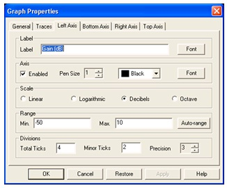
Figure 4.31.

Setting the Graph Properties for the Magnitude

1. 1. 1. In the Divisions section, choose Total Ticks of 4, Minor Ticks of 2 and Precision of 3.

2. Click the Apply button.

2. Select the Bottom Axis tab.

1. Select Logarithmic Scale. In the Frequency Range, type 1000 for minimum and 1000000 for maximum.
2. Click Apply, then OK.

2. Adjust the bottom (Phase) graph by setting the Graph Properties as shown in the following figure. Then click on the Bottom Axis tab and change the range to 1000 to 1000000.

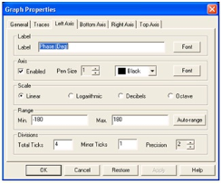
Figure 4.32.

Setting the Graph Properties for the Phase

Now compare the outputs of the Bode plot and the AC analysis by directly overlaying the magnitude traces.

1. Left-click on the magnitude plot of the Bode plot to select it.

1. Select Overlay Traces from the Tools menu.
2. Pick Graph_1 of the AC Analysis (this should be the second last entry in the list).

A new page will open in the Grapher that displays the two traces overlaid.

You can zoom in to see the region where both traces exist. Press and hold the left mouse button as you drag a box around the peak of the graph.

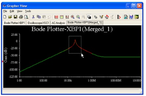
Figure 4.33.

Zooming in on Overlaid Traces

Notice the results are slightly different. This is because the two methods used different sampling rates. You can control the sampling rate when you set up the instrument or the analysis.

1. Investigate how to make precise measurements in the Grapher.

1. Select the Bode Plot Tab in the Grapher.
2. Turn on the cursors by selecting Show/Hide Cursors from the Viewmenu.
3. Select one of the cursors and right-click on it.
4. Select Go to next Y_MAX to find the peak.
5. Select Set Y_Value =>and enter the value that is 3 less than the max. This will give you one of the -3dB points.
6. Read the resulting value in the numeric display box.

2. Perform Transient Analysis (Simulate/Analyses/Transient Analysis).

1. Set the analysis settings as shown below. Note: You may need to expand the dialog box by clicking the More button.

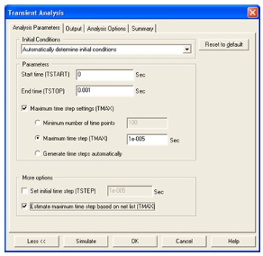
Figure 4.34.

Setting Up the Transient Analysis

1. 1. Switch to the Outputtab.

2. Select test point nodes $input and $output as the Selected Variables for Analysis.

3. Click the Simulate button. Compare the graph with the oscilloscope display.

You will now set up to run a Fourier analysis.

1. Open the instrument panel of the function generator and change the waveform to a square wave.

1. Choose Simulate/Analyses/Fourier Analysis.
2. Select both Estimate buttons to set the sampling options and transient Analysis options automatically.
3. Switch to the Outputvariablestab.
4. Select $input and $output as the Selected Variables for Analysis.
5. Click Simulate.

Note the output is presented on two separate pages in the Grapher.

Optional Section (time permitting):

Perform a Monte Carlo Analysis, (Simulate/Analyses/Monte Carlo).

1. From the front dialog box, select Add a new tolerance function.

1. In Parameter Type, choose Device Parameter.
2. In Device Type select Capacitor. Choose cc1.
3. In the Tolerance section, select Percent. For Tolerance Type, assign 20 and click Accept.

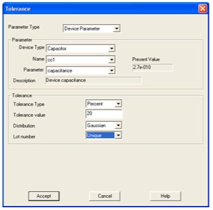
Figure 4.35.

Setting Device Tolerances

1. 1. Select Add a new tolerance again, and repeat the above procedure. Select cc2 this time.

2. Now configure the Analysis Parameters.

3. Click on the Analysis Parameters tab.

4. Set it up to run an AC Analysis, with 5 runs, and set the Output variable to $output.

5. Click on the Edit Analysis button and then configure the settings for the AC analysis.

6. Set the FSTART to 1 kHz, the FSTOP to 1 MHz, the Number of points per decade to 100 and the Vertical scale to Decibel.

7. Click the Simulate button.

SOLUTION

Solutions