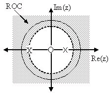
Figure 3.18.
The ROC of
Once again, by linearity,
()
By observation it is again clear that there are two zeros, at 0 and , and two poles, at , and
. in ths case though, the ROC is
.
Figure 3.19.
The ROC of
.
Graphical Understanding of ROC


Using the demonstration, learn about the region of convergence for the Laplace Transform.
Conclusion
Clearly, in order to craft a system that is actually useful by virtue of being causal and BIBO
stable, we must ensure that it is within the Region of Convergence, which can be ascertained by
looking at the pole zero plot. The Region of Convergence is the area in the pole/zero plot of the
transfer function in which the function exists. For purposes of useful filter design, we prefer to
work with rational functions, which can be described by two polynomials, one each for
determining the poles and the zeros, respectively.
3.8. Understanding Pole/Zero Plots on the Z-Plane*
Introduction to Poles and Zeros of the Z-Transform
It is quite difficult to qualitatively analyze the Laplace transform and Z-transform, since mappings of their magnitude and phase or real part and imaginary part result in multiple
mappings of 2-dimensional surfaces in 3-dimensional space. For this reason, it is very common to
examine a plot of a transfer function's poles and zeros to try to gain a qualitative idea of what a system does.
Once the Z-transform of a system has been determined, one can use the information contained in
function's polynomials to graphically represent the function and easily observe many defining
characteristics. The Z-transform will have the below structure, based on Rational Functions: ()
The two polynomials, P( z) and Q( z), allow us to find the poles and zeros of the Z-Transform.
Definition: zeros
1. The value(s) for z where
.
2. The complex frequencies that make the overall gain of the filter transfer function zero.
Definition: poles
1. The value(s) for z where
.
2. The complex frequencies that make the overall gain of the filter transfer function infinite.


Example 3.8.
Below is a simple transfer function with the poles and zeros shown below it.
The zeros are: {–1}
The poles are:
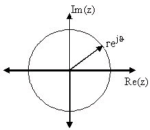
The Z-Plane
Once the poles and zeros have been found for a given Z-Transform, they can be plotted onto the Z-
Plane. The Z-plane is a complex plane with an imaginary and real axis referring to the complex-
valued variable z. The position on the complex plane is given by rⅇⅈθ and the angle from the positive, real axis around the plane is denoted by θ. When mapping poles and zeros onto the plane,
poles are denoted by an "x" and zeros by an "o". The below figure shows the Z-Plane, and
examples of plotting zeros and poles onto the plane can be found in the following section.
Figure 3.20. Z-Plane
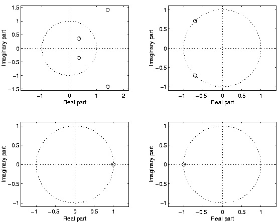
Examples of Pole/Zero Plots
This section lists several examples of finding the poles and zeros of a transfer function and then
plotting them onto the Z-Plane.
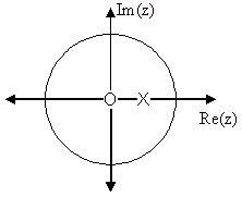
Example 3.9. Simple Pole/Zero Plot
The zeros are: {0}
The poles are:
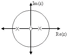


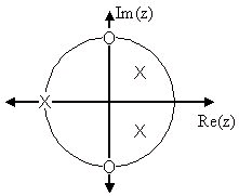


Figure 3.21. Pole/Zero Plot
Using the zeros and poles found from the transfer function, the one zero is mapped to zero and the two poles are placed at and Example 3.10. Complex Pole/Zero Plot
The zeros are: { ⅈ, – ⅈ}
The poles are:
Figure 3.22. Pole/Zero Plot
Using the zeros and poles found from the transfer function, the zeros are mapped to ± ⅈ, and the poles are placed at –1, and
Example 3.11. Pole-Zero Cancellation
An easy mistake to make with regards to poles and zeros is to think that a function like
is the same as s+3 . In theory they are equivalent, as the pole and zero at s=1 cancel
each other out in what is known as pole-zero cancellation. However, think about what may
happen if this were a transfer function of a system that was created with physical circuits. In
this case, it is very unlikely that the pole and zero would remain in exactly the same place. A

minor temperature change, for instance, could cause one of them to move just slightly. If this
were to occur a tremendous amount of volatility is created in that area, since there is a change
from infinity at the pole to zero at the zero in a very small range of signals. This is generally a
very bad way to try to eliminate a pole. A much better way is to use control theory to move
the pole to a better place.
Repeated Poles and Zeros
It is possible to have more than one pole or zero at any given point. For instance, the discrete-
time transfer function H( z)= z 2 will have two zeros at the origin and the continuous-time
function
will have 25 poles at the origin.
MATLAB - If access to MATLAB is readily available, then you can use its functions to easily
create pole/zero plots. Below is a short program that plots the poles and zeros from the above
example onto the Z-Plane.
% Set up vector for zeros
z = [j ; -j];
% Set up vector for poles
p = [-1 ; .5+.5j ; .5-.5j];
figure(1);
zplane(z,p);
title('Pole/Zero Plot for Complex Pole/Zero Plot Example');
Interactive Demonstration of Poles and Zeros
Figure 3.23.
Interact (when online) with a Mathematica CDF demonstrating Pole/Zero Plots. To Download, right-click and save target as .cdf.
Applications for pole-zero plots
Stability and Control theory
Now that we have found and plotted the poles and zeros, we must ask what it is that this plot gives
us. Basically what we can gather from this is that the magnitude of the transfer function will be
larger when it is closer to the poles and smaller when it is closer to the zeros. This provides us
with a qualitative understanding of what the system does at various frequencies and is crucial to
the discussion of stability.
Pole/Zero Plots and the Region of Convergence
The region of convergence (ROC) for X( z) in the complex Z-plane can be determined from the
pole/zero plot. Although several regions of convergence may be possible, where each one
corresponds to a different impulse response, there are some choices that are more practical. A
ROC can be chosen to make the transfer function causal and/or stable depending on the pole/zero
plot.
Filter Properties from ROC
If the ROC extends outward from the outermost pole, then the system is causal.

If the ROC includes the unit circle, then the system is stable.
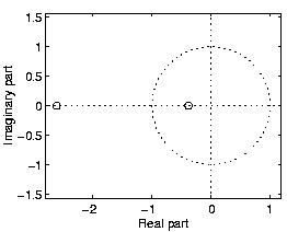
Below is a pole/zero plot with a possible ROC of the Z-transform in the Simple Pole/Zero Plot
discussed earlier. The shaded region indicates the ROC chosen for the filter. From this figure, we
can see that the filter will be both causal and stable since the above listed conditions are both met.
Example 3.12.
Figure 3.24. Region of Convergence for the Pole/Zero Plot
The shaded area represents the chosen ROC for the transfer function.
Frequency Response and Pole/Zero Plots
The reason it is helpful to understand and create these pole/zero plots is due to their ability to help
us easily design a filter. Based on the location of the poles and zeros, the magnitude response of
the filter can be quickly understood. Also, by starting with the pole/zero plot, one can design a
filter and obtain its transfer function very easily.
3.9. Zero Locations of Linear-Phase FIR Filters*
Zero Locations of Linear-Phase Filters
The zeros of the transfer function H( z) of a linear-phase filter lie in specific configurations.
We can write the symmetry condition h( n)= h( N−(1− n)) in the Z domain. Taking the Z-transform


of both sides gives
()
Recall that we are assuming that h( n) is real-valued. If z 0 is a zero of H( z) , H( z 0)=0 then (Because the roots of a polynomial with real coefficients exist in complex-conjugate pairs.)
Using the symmetry condition, Equation, it follows that
and
or
If z 0 is a zero of a (real-valued) linear-phase filter, then so are , , and .
ZEROS LOCATIONS
It follows that
1. generic zeros of a linear-phase filter exist in sets of 4.
2. zeros on the unit circle ( z 0= ⅇⅈω 0 ) exist in sets of 2. ( z 0≠±1 )
3. zeros on the real line ( z 0= a ) exist in sets of 2. ( z 0≠±1 )
4. zeros at 1 and -1 do not imply the existence of zeros at other specific points.
(a)
(b)
Figure 3.25.
Examples of zero sets
ZERO LOCATIONS: AUTOMATIC ZEROS
The frequency response Hf( ω) of a Type II FIR filter always has a zero at ω= π :
h( n)=[ h 0, h 1, h 2, h 2, h 1, h 0] H( z)= h 0+ h 1 z-1+ h 2 z-2+ h 2 z-3+ h 1 z-4+ h 0 z-5 H(-1)= h 0− h 1+ h 2− h 2+ h 1− h 0=0
Hf( π)= H( ⅇⅈπ)= H(-1)=0
Rule
Hf( π)=0
Similarly, we can derive the following rules for Type III and Type IV FIR filters.
Rule
Hf(0)= Hf( π)=0
Rule
Hf(0)=0
The automatic zeros can also be derived using the characteristics of the amplitude response
A( ω) seen earlier.
Table 3.2.
Type automatic zeros
I
—
II
ω= π
III
ω=0 or π
IV
ω=0
ZERO LOCATIONS: EXAMPLES
The Matlab command zplane can be used to plot the zero locations of FIR filters.
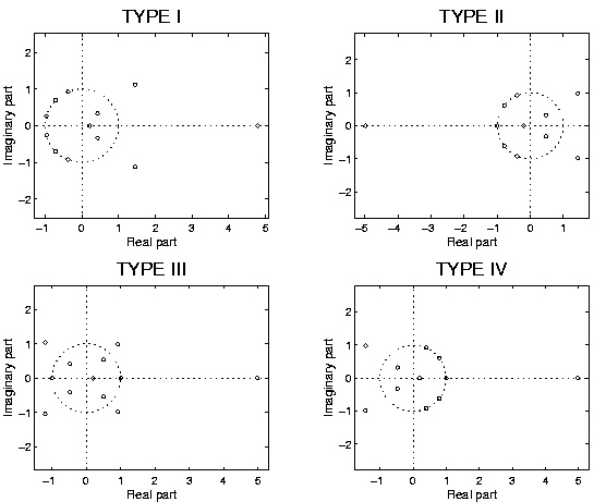

Figure 3.26.
Note that the zero locations satisfy the properties noted previously.
3.10. Discrete Time Filter Design*
Estimating Frequency Response from Z-Plane
One of the primary motivating factors for utilizing the z-transform and analyzing the pole/zero
plots is due to their relationship to the frequency response of a discrete-time system. Based on the
position of the poles and zeros, one can quickly determine the frequency response. This is a result
of the correspondence between the frequency response and the transfer function evaluated on the
unit circle in the pole/zero plots. The frequency response, or DTFT, of the system is defined as:
()


Next, by factoring the transfer function into poles and zeros and multiplying the numerator and
denominator by ⅇⅈw we arrive at the following equations:
()
From Equation we have the frequency response in a form that can be used to interpret physical characteristics about the filter's frequency response. The numerator and denominator contain a
product of terms of the form | ⅇⅈw− h|, where h is either a zero, denoted by ck or a pole, denoted by dk. Vectors are commonly used to represent the term and its parts on the complex plane. The pole
or zero, h, is a vector from the origin to its location anywhere on the complex plane and ⅇⅈw is a vector from the origin to its location on the unit circle. The vector connecting these two points,
| ⅇⅈw− h|, connects the pole or zero location to a place on the unit circle dependent on the value of w. From this, we can begin to understand how the magnitude of the frequency response is a ratio
of the distances to the poles and zero present in the z-plane as w goes from zero to pi. These
characteristics allow us to interpret | H( w)| as follows:
()
Drawing Frequency Response from Pole/Zero Plot
Let us now look at several examples of determining the magnitude of the frequency response from
the pole/zero plot of a z-transform. If you have forgotten or are unfamiliar with pole/zero plots,
please refer back to the Pole/Zero Plots module.
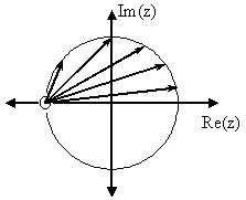
Example 3.13.
In this first example we will take a look at the very simple z-transform shown below:
H( z)= z+1=1+ z-1 H( w)=1+ ⅇ–( ⅈw) For this example, some of the vectors represented by | ⅇⅈw− h|, for random values of w, are explicitly drawn onto the complex plane shown in the figure
below. These vectors show how the amplitude of the frequency response changes as w goes
from 0 to 2 π, and also show the physical meaning of the terms in Equation above. One can see that when w=0, the vector is the longest and thus the frequency response will have its largest
amplitude here. As w approaches π, the length of the vectors decrease as does the amplitude of
| H( w)|. Since there are no poles in the transform, there is only this one vector term rather than
a ratio as seen in Equation.
<db:title>Pole/Zero Plot</db:title>
<db:title>Frequency Response: |H(w)|</db:title>


(a)
(b)
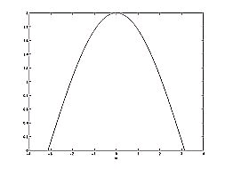
Figure 3.27.
The first figure represents the pole/zero plot with a few representative vectors graphed while the second shows the frequency response with a peak at +2 and graphed between plus and minus π.
Example 3.14.
For this example, a more complex transfer function is analyzed in order to represent the
system's frequency response.
Below we can see the two figures described by the above equations. The Figure 3.28a
represents the basic pole/zero plot of the z-transform, H( w). Figure 3.28b shows the magnitude of the frequency response. From the formulas and statements in the previous section, we can
see that when w=0 the frequency will peak since it is at this value of w that the pole is closest
to the unit circle. The ratio from Equation helps us see the mathematics behind this conclusion and the relationship between the distances from the unit circle and the poles and zeros. As w
moves from 0 to π, we see how the zero begins to mask the effects of the pole and thus force
the frequency response closer to 0.
<db:title>Pole/Zero Plot</db:title>
<db:title>Frequency Response: |H(w)|</db:title>
(a)
(b)
Figure 3.28.
The first figure represents the pole/zero plot while the second shows the frequency response with a peak at +2 and graphed between plus and minus π.
Interactive Filter Design Illustration
(This media type is not supported in this reader. Click to open media in browser.)
Figure 3.29.
Digital filter design LabVIEW virtual instrument by NI from http://cnx.org/content/m13115/latest/.
Conclusion
In conclusion, using the distances from the unit circle to the poles and zeros, we can plot the
frequency response of the system. As w goes from 0 to 2 π , the following two properties, taken
from the above equations, specify how one should draw | H( w)|.
While moving around the unit circle...
1. if close to a zero, then the magnitude is small. If a zero is on the unit circle, then the frequency
response is zero at that point.
2. if close to a pole, then the magnitude is large. If a pole is on the unit circle, then the frequency
response goes to infinity at that point.
Glossary
Definition: Complex Plane
A two-dimensional graph where the horizontal axis maps the real part and the vertical axis
maps the imaginary part of any complex number or function.
Definition: difference equation
An equation that shows the relationship between consecutive values of a sequence and the
differences among them. They are often rearranged as a recursive formula so that a systems
output can be computed from the input signal and past outputs. Example .
simplemath mathml-miitalicsy[ mathml-miitalicsn]+7 mathml-miitalicsy[ mathml-miitalicsn−1]+2
Definition: domain
The group, or set, of values that are defined by a given function. Example . Using the
rational function above, ???, the domain can be defined as any real number
simplemath mathml-miitalicsx x where simplemath mathml-miitalicsx x does not
equal 1 or negative 3. Written out mathematical, we get the following:
Definition: poles
1. The value(s) for simplemath mathml-miitalicsz z where the bolddenominator of the transfer
function equals zero
2. The complex frequencies that make the overall gain of the filter transfer function infinite.
Definition: poles
1. The value(s) for simplemath mathml-miitalicsz z where Qz= .
2. The complex frequencies that make the overall gain of the filter transfer function infinite.
Definition: rational function
For any two polynomials, A and B, their quotient is called a rational function. Example .
Below is a simple example of a basic rational function,
simplemath mathml-miitalicsf( mathml-miitalicsx) fx . Note that the
numerator and denominator can be polynom