Hf( ω)= A( ω) ⅇⅈθ( ω)
()
θ( ω)=(– M) ω
TYPE III: ODD-LENGTH ANTI-SYMMETRIC
The frequency response of a length N=5 FIR Type III filter can be written as follows.
()
()
()
Hf( ω)= ⅇ-2 ⅈω( h 0( ⅇ 2 ⅈω− ⅇ-2 ⅈω)+ h 1( ⅇⅈω− ⅇ(– ⅈ) ω)) ()
Hf( ω)= ⅇ-2 ⅈω(2 ⅈh 0sin(2 ω)+2 ⅈh 1sin( ω))
()
Hf( ω)= ⅇ-2 ⅈωⅈ(2 h 0sin(2 ω)+2 h 1sin( ω))
()
()
Hf( ω)= A( ω) ⅇⅈθ( ω)
where
A( ω)=2 h 0sin(2 ω)+2 h 1sin( ω) In general, for a Type III FIR filters of length N: Hf( ω)= A( ω) ⅇⅈθ( ω)
()
TYPE IV: EVEN-LENGTH ANTI-SYMMETRIC
The frequency response of a length N=4 FIR Type IV filter can be written as follows.
()
()


()
()
()
()
()
Hf( ω)= A( ω) ⅇⅈθ( ω)
where
In general, for a Type IV FIR filters of length N:
Hf( ω)= A( ω) ⅇⅈθ( ω)
()
5.3. Design of Linear-Phase FIR Filters by DFT-Based
Interpolation*
DESIGN OF FIR FILTERS BY DFT-BASED INTERPOLATION
One approach to the design of FIR filters is to ask that A( ω) pass through a specified set of values.
If the number of specified interpolation points is the same as the number of filter parameters, then
the filter is totally determined by the interpolation conditions, and the filter can be found by
solving a system of linear equations. When the interpolation points are equally spaced between 0
and 2 π , then this interpolation problem can be solved very efficiently using the DFT.
To derive the DFT solution to the interpolation problem, recall the formula relating the samples of
the frequency response to the DFT. In the case we are interested here, the number of samples is to
be the same as the length of the filter ( L= N ).
()


Types I and II
Recall the relation between A( ω) and Hf( ω) for a Type I and II filter, to obtain
()
Now we can related the N-point DFT of h( n) to the samples of A( ω) :
Finally,
we can solve for the filter coefficients h( n) .
()
Therefore, if the values
are specified, we can then obtain the filter coefficients h( n) that
satisfies the interpolation conditions by using the inverse DFT. It is important to note however,
that the specified values
must possess the appropriate symmetry in order for the result of the
inverse DFT to be a real Type I or II FIR filter.
Types III and IV
For Type III and IV filters, we have
()
Then we can related the N-point DFT of h( n) to the samples of A( ω) :
Solving
for the filter coefficients h( n) gives:
()
EXAMPLE: DFT-INTERPOLATION (TYPE I)
The following Matlab code fragment illustrates how to use this approach to design a length 11
Type I FIR filter for which
.
>> N = 11;
>> M = (N-1)/2;
>> Ak = [1 1 1 0 0 0 0 0 0 1 1}; % samples of A(w)
>> k = 0:N-1;
>> W = exp(j*2*pi/N);
>> h = ifft(Ak.*W.^(-M*k));
>> h'
ans =
0.0694 - 0.0000i
-0.0540 - 0.0000i
-0.1094 + 0.0000i
0.0474 + 0.0000i
0.3194 + 0.0000i
0.4545 + 0.0000i
0.3194 + 0.0000i
0.0474 + 0.0000i
-0.1094 + 0.0000i
-0.0540 - 0.0000i
0.0694 - 0.0000i
Observe that the filter coefficients h are real and symmetric; that a Type I filter is obtained as
desired. The plot of A( ω) for this filter illustrates the interpolation points.
L = 512;
H = fft([h zeros(1,L-N)]);
W = exp(j*2*pi/L);
k = 0:L-1;
A = H .* W.^(M*k);
A = real(A);
w = k*2*pi/L;
plot(w/pi,A,2*[0:N-1]/N,Ak,'o')
xlabel('\omega/\pi')
title('A(\omega)')
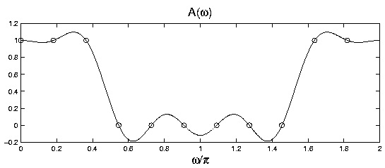


Figure 5.5.
An exercise for the student: develop this DFT-based interpolation approach for Type II, III, and IV
FIR filters. Modify the Matlab code above for each case.
SUMMARY: IMPULSE AND AMP RESPONSE
For an N-point linear-phase FIR filter h( n) , we summarize:
1. The formulas for evaluating the amplitude response A( ω) at L equally spaced points from 0 to 2 π ( L≥ N ).
2. The formulas for the DFT-based interpolation design of h( n) .
TYPE I and II:
()
()
TYPE III and IV:
()
()
5.4. Design of Linear-Phase FIR Filters by General
Interpolation*


DESIGN OF FIR FILTERS BY GENERAL INTERPOLATION
If the desired interpolation points are not uniformly spaced between 0 and π then we can not use
the DFT. We must take a different approach. Recall that for a Type I FIR filter,
For convenience, it is common to write this as
where h( M)= a(0) and
. Note that there are M+1 parameters. Suppose it is
desired that A( ω) interpolates a set of specified values: A( ωk)= Ak , 0≤ k≤ M To obtain a Type I FIR filter satisfying these interpolation equations, one can set up a linear system of equations.
In matrix form, we have
Once
a( n) is found, the filter h( n) is formed as
{ h( n)}=1/2{ a( M), a( M−1), …, a(1), 2 a(0), a(1), …, a( M−1), a( M)}
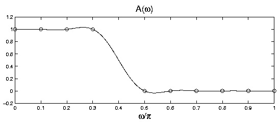
EXAMPLE
In the following example, we design a length 19 Type I FIR. Then M=9 and we have 10
parameters. We can therefore have 10 interpolation equations. We choose:
()
A( ωk)=1 , ωk={0, 0.1 π, 0.2 π, 0.3 π} 0≤ k≤3
()
A( ωk)=0 , ωk={0.5 π, 0.6 π, 0.7 π, 0.8 π, 0.8 π, 1.0 π} 4≤ k≤9
To solve this interpolation problem in Matlab, note that the matrix can be generated by a single
multiplication of a column vector and a row vector. This is done with the command C =
cos(wk*[0:M]); where wk is a column vector containing the frequency points. To solve the
linear system of equations, we can use the Matlab backslash command.
N = 19;
M = (N-1)/2;
wk = [0 .1 .2 .3 .5 .6 .7 .8 .9 1]'*pi;
Ak = [1 1 1 1 0 0 0 0 0 0]';
C = cos(wk*[0:M]);
a = C/Ak;
h = (1/2)*[a([M:-1:1]+1); 2*a([0]+1); a(1:M]+1)];
[A,w] = firamp(h,1);
plot(w/pi,A,wk/pi,Ak,'o')
title('A(\omega)')
xlabel('\omega/\pi')
Figure 5.6.
The general interpolation problem is much more flexible than the uniform interpolation problem
that the DFT solves. For example, by leaving a gap between the pass-band and stop-band as in this
example, the ripple near the band edge is reduced (but the transition between the pass- and stop-
bands is not as sharp). The general interpolation problem also arises as a subproblem in the design
of optimal minimax (or Chebyshev) FIR filters.
LINEAR-PHASE FIR FILTERS: PROS AND CONS
FIR digital filters have several desirable properties.
They can have exactly linear phase.
They can not be unstable.
There are several very effective methods for designing linear-phase FIR digital filters.
On the other hand,
Linear-phase filters can have long delay between input and output.
If the phase need not be linear, then IIR filters can be more efficient.
5.5. Linear-Phase FIR Filters: Amplitude Formulas*


SUMMARY: AMPLITUDE FORMULAS
Table 5.2.
Type
θ( ω)
A( ω)
I
–( Mω)
II
–( Mω)
III
IV
where
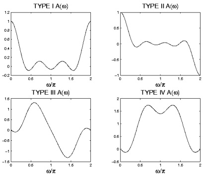
AMPLITUDE RESPONSE CHARACTERISTICS
To analyze or design linear-phase FIR filters, we need to know the characteristics of the amplitude
response A( ω) .
Table 5.3.
Type Properties
A( ω) is even about
A( ω)= A(– ω)
ω=0
A( ω) is even about
I
A( π+ ω)= A( π− ω)
ω= π
A( ω) is periodic with
A( ω+2 π)= A( ω)
2 π
A( ω) is even about
A( ω)= A(– ω)
ω=0
II
A( ω) is odd about ω= π
A( π+ ω)=–( A( π− ω))


A( ω) is periodic with
A( ω+4 π)= A( ω)
4 π
A( ω) is odd about ω=0
A( ω)=–( A(– ω))
A( ω) is odd about ω= π
A( π+ ω)=–( A( π− ω))
III
A( ω) is periodic with
A( ω+2 π)= A( ω)
2 π
A( ω) is odd about ω=0
A( ω)=–( A(– ω))
A( ω) is even about
A( π+ ω)= A( π− ω)
IV
ω= π
A( ω) is periodic with
A( ω+4 π)= A( ω)
4 π
Figure 5.7.
EVALUATING THE AMPLITUDE RESPONSE
The frequency response Hf( ω) of an FIR filter can be evaluated at L equally spaced frequencies between 0 and π using the DFT. Consider a causal FIR filter with an impulse response h( n) of length- N, with N≤ L . Samples of the frequency response of the filter can be written as
Define the L-point signal { g( n)|0≤ n≤ L−1} as
Then


where G( k) is the L-point DFT of g( n) .
Types I and II
Suppose the FIR filter h( n) is either a Type I or a Type II FIR filter. Then we have from above
Hf( ω)= A( ω) ⅇ(– ⅈ) Mω or A( ω)= Hf( ω) ⅇⅈMω Samples of the real-valued amplitude A( ω) can be obtained from samples of the function Hf( ω) as:
Therefore, the samples
of the real-valued amplitude function can be obtained by zero-padding h( n) , taking the DFT, and
multiplying by the complex exponential. This can be written as:
()
Types III and IV
For Type III and Type IV FIR filters, we have Hf( ω)= ⅈⅇ(– ⅈ) MωA( ω) or A( ω)=(– ⅈ) Hf( ω) ⅇⅈMω Therefore, samples of the real-valued amplitude A( ω) can be obtained from samples of the function Hf( ω) as:
Therefore, the samples of the
real-valued amplitude function can be obtained by zero-padding h( n) , taking the DFT, and
multiplying by the complex exponential.
()
Example 5.1. EVALUATING THE AMP RESP (TYPE I)
In this example, the filter is a Type I FIR filter of length 7. An accurate plot of A( ω) can be
obtained with zero padding.
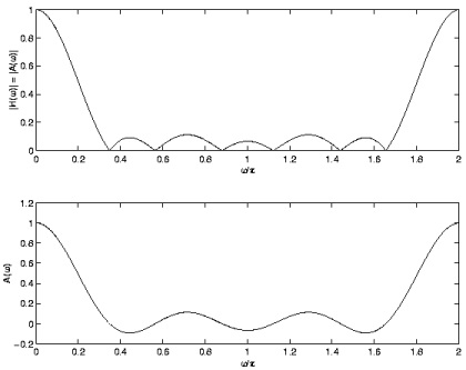
Figure 5.8.
The following Matlab code fragment for the plot of A( ω) for a Type I FIR filter.
h = [3 4 5 6 5 4 3]/30;
N = 7;
M = (N-1)/2;
L = 512;
H = fft([h zeros(1,L-N)]);
k = 0:L-1;
W = exp(j*2*pi/L);
A = H .* W.^(M*k);
A = real(A);
figure(1)
w = [0:L-1]*2*pi/(L-1);
subplot(2,1,1)
plot(w/pi,abs(H))
ylabel('|H(\omega)| = |A(\omega)|')
xlabel('\omega/\pi')
subplot(2,1,2)
plot(w/pi,A)
ylabel('A(\omega)')
xlabel('\omega/\pi')
print -deps type1
The command A = real(A) removes the imaginary part which is equal to zero to within
computer precision. Without this command, Matlab takes A to be a complex vector and the
following plot command will not be right.
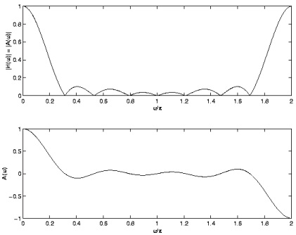
Observe the symmetry of A( ω) due to h( n) being real-valued. Because of this symmetry, A( ω) is usually plotted for 0≤ ω≤ π only.
Example 5.2. EVALUATING THE AMP RESP (TYPE II)
Figure 5.9.
The following Matlab code fragment produces a plot of A( ω) for a Type II FIR filter.
h = [3 5 6 7 7 6 5 3]/42;
N = 8;
M = (N-1)/2;
L = 512;
H = fft([h zeros(1,L-N)]);
k = 0:L-1;
W = exp(j*2*pi/L);
A = H .* W.^(M*k);
A = real(A);
figure(1)
w = [0:L-1]*2*pi/(L-1);
subplot(2,1,1)
plot(w/pi,abs(H))
ylabel('|H(\omega)| = |A(\omega)|')
xlabel('\omega/\pi')
subplot(2,1,2)
plot(w/pi,A)
ylabel('A(\omega)')
xlabel('\omega/\pi')
print -deps type2
The imagin