Using what we know about Hilbert spaces: For any f( t)∈ L 2([ 0, T]) , we can write (8.3)
Synthesis
(8.4)
Analysis

()
the w j , k are real
The Haar transform is super useful especially in image compression
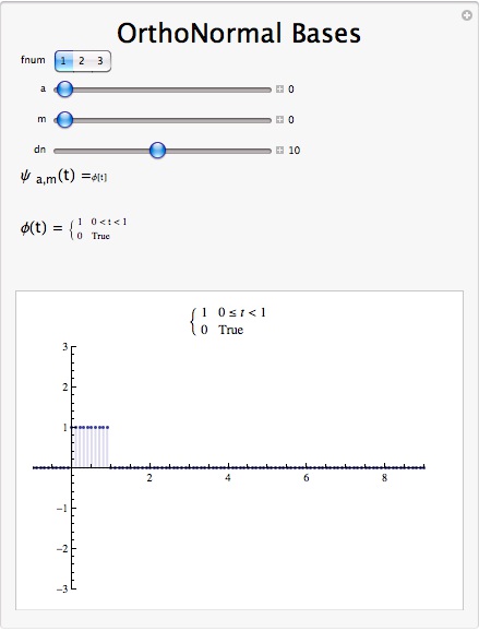
Haar Wavelet Demonstration
Figure 8.10.
Interact (when online) with a Mathematica CDF demonstrating the Haar Wavelet as an Orthonormal Basis.
8.2. Orthonormal Wavelet Basis*


An orthonormal wavelet basis is an orthonormal basis of the form
()
The function ψ( t) is called the wavelet.
The problem is how to find a function ψ( t) so that the set B is an orthonormal set.
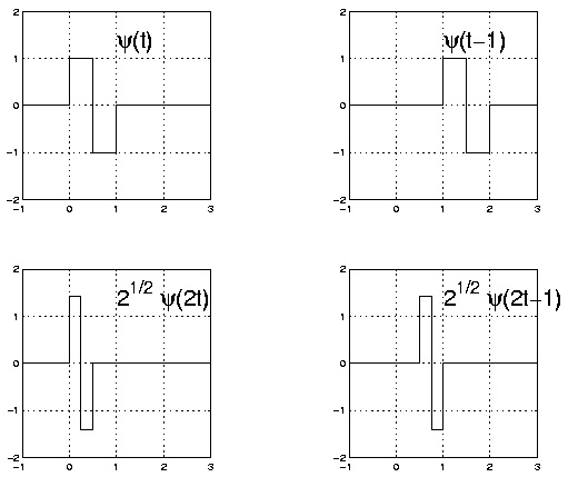
Example 8.1. Haar Wavelet
The Haar basis (described by Haar in 1910) is an orthonormal basis with wavelet ψ( t) ()
For the Haar wavelet, it is easy to verify that the set B is an orthonormal set (Figure 8.11).
Figure 8.11.
Notation:
where j is an index of scale and k is an index of location.
If B is an orthonormal set then we have the wavelet series.


(8.5)
Wavelet series
8.3. Continuous Wavelet Transform*
The STFT provided a means of (joint) time-frequency analysis with the property that
spectral/temporal widths (or resolutions) were the same for all basis elements. Let's now take a
closer look at the implications of uniform resolution.
Consider two signals composed of sinusoids with frequency 1 Hz and 1.001 Hz, respectively. It
may be difficult to distinguish between these two signals in the presence of background noise
unless many cycles are observed, implying the need for a many-second observation. Now consider
two signals with pure frequencies of 1000 Hz and 1001 Hz-again, a 0.1% difference. Here it should
be possible to distinguish the two signals in an interval of much less than one second. In other
words, good frequency resolution requires longer observation times as frequency decreases. Thus,
it might be more convenient to construct a basis whose elements have larger temporal width at
low frequencies.
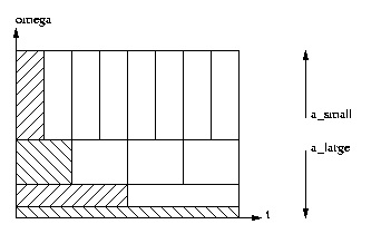
The previous example motivates a multi-resolution time-frequency tiling of the form
Figure 8.12.
The Continuous Wavelet Transform (CWT) accomplishes the above multi-resolution tiling by
time-scaling and time-shifting a prototype function ψ( t) , often called the mother wavelet. The a-
scaled and τ-shifted basis elements is given by
where a and τ∈ℝ


The conditions above imply that ψ( t) is bandpass and sufficiently smooth.
Assuming that ∥ ψ( t)∥=1 , the definition above ensures that ∥ ψ a , τ ( t)∥=1 for all a and τ. The CWT
is then defined by the transform pair
In
basis terms, the CWT says that a waveform can be decomposed into a collection of shifted and
stretched versions of the mother wavelet ψ( t) . As such, it is usually said that wavelets perform a
"time-scale" analysis rather than a time-frequency analysis.
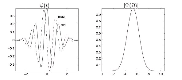
The Morlet wavelet is a classic example of the CWT. It employs a windowed complex
exponential as the mother wavelet:
where it is typical to select
. (See illustration.) While this wavelet does not exactly satisfy the conditions established earlier, since Ψ(0)≈7×10⁻⁷≠0 , it can be corrected, though in practice the correction is
negligible and usually ignored.
Figure 8.13.
While the CWT discussed above is an interesting theoretical and pedagogical tool, the discrete
wavelet transform (DWT) is much more practical. Before shifting our focus to the DWT, we take
a step back and review some of the basic concepts from the branch of mathematics known as
Hilbert Space theory (Vector Space, Normed Vector Space, Inner Product Space, Hilbert
Space, Projection Theorem). These concepts will be essential in our development of the DWT.
8.4. Discrete Wavelet Transform: Main Concepts*


Main Concepts
The discrete wavelet transform (DWT) is a representation of a signal x( t)∈ ℒ 2 using an orthonormal basis consisting of a countably-infinite set of wavelets. Denoting the wavelet basis as
, the DWT transform pair is
()
()
where { d k , n } are the wavelet coefficients. Note the relationship to Fourier series and to the sampling theorem: in both cases we can perfectly describe a continuous-time signal x( t) using a
countably-infinite ( i.e. , discrete) set of coefficients. Specifically, Fourier series enabled us to
describe periodic signals using Fourier coefficients { X[ k]| k∈ℤ} , while the sampling theorem enabled us to describe bandlimited signals using signal samples { x[ n]| n∈ℤ} . In both cases, signals within a limited class are represented using a coefficient set with a single countable index.
The DWT can describe any signal in ℒ 2 using a coefficient set parameterized by two countable
indices:
.
Wavelets are orthonormal functions in ℒ 2 obtained by shifting and stretching a mother wavelet, ψ( t)∈ ℒ 2 . For example,
()
defines a family of wavelets
related by power-of-two stretches. As k
increases, the wavelet stretches by a factor of two; as n increases, the wavelet shifts right.
When ∥ ψ( t)∥=1 , the normalization ensures that ∥ ψ k , n ( t)∥=1 for all k∈ℤ , n∈ℤ .
Power-of-two stretching is a convenient, though somewhat arbitrary, choice. In our treatment of
the discrete wavelet transform, however, we will focus on this choice. Even with power-of two
stretches, there are various possibilities for ψ( t) , each giving a different flavor of DWT.
Wavelets are constructed so that
( i.e. , the set of all shifted wavelets at fixed scale k),
describes a particular level of 'detail' in the signal. As k becomes smaller ( i.e. , closer to –∞ ), the wavelets become more "fine grained" and the level of detail increases. In this way, the DWT can
give a multi-resolution description of a signal, very useful in analyzing "real-world" signals.


Essentially, the DWT gives us a discrete multi-resolution description of a continuous-time
signal in ℒ 2 .
In the modules that follow, these DWT concepts will be developed "from scratch" using Hilbert
space principles. To aid the development, we make use of the so-called scaling function
φ( t)∈ ℒ 2 , which will be used to approximate the signal up to a particular level of detail. Like with wavelets, a family of scaling functions can be constructed via shifts and power-of-two
stretches
()
given mother scaling function φ( t) . The relationships between wavelets and scaling functions will be elaborated upon later via theory and example.
The inner-product expression for d k , n , Equation is written for the general complex-valued case. In our treatment of the discrete wavelet transform, however, we will assume real-valued
signals and wavelets. For this reason, we omit the complex conjugations in the remainder of
our DWT discussions
8.5. The Haar System as an Example of DWT*
The Haar basis is perhaps the simplest example of a DWT basis, and we will frequently refer to it
in our DWT development. Keep in mind, however, that the Haar basis is only an example; there
are many other ways of constructing a DWT decomposition.
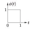
For the Haar case, the mother scaling function is defined by Equation and Figure 8.14.
()
Figure 8.14.

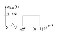

From the mother scaling function, we define a family of shifted and stretched scaling functions
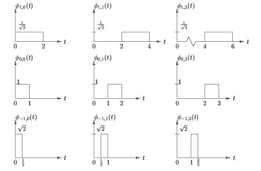
{ φ k , n ( t)} according to Equation and Figure 8.15
()
Figure 8.15.
which are illustrated in Figure 8.16 for various k and n. Equation makes clear the principle that incrementing n by one shifts the pulse one place to the right. Observe from Figure 8.16 that is orthonormal for each k ( i.e. , along each row of figures).
Figure 8.16.
Solutions
Index
A
amplitude response, THE AMPLITUDE RESPONSE
analog-to-digital (a/d) conversion, Amplitude Quantization
autocorrelation, Autocorrelation Function, Glossary
average power, Mean-Square Value
B
bandlimited, Sampling Period/Rate, Main Concepts
ber, Example - Detection of a binary signal in noise
bilateral z-transform, Basic Definition of the Z-Transform
bilinear transform, Bilinear Transform
bit error rate, Example - Detection of a binary signal in noise
C
causal, Pole/Zero Plots and the Region of Convergence
characteristic polynomial, Homogeneous Solution
circular convolution, Compute IDFT of Y[k]
complex plane, Complex Plane, Glossary
computational algorithm, The FFT Algorithm, Glossary
continuous random process, Random Process
control theory, Pole-Zero Cancellation, Examples of Pole/Zero Plots
correlation, Correlation, Glossary
correlation coefficient, Correlation Coefficient
correlation functions, Correlation
covariance, Covariance, Glossary
crosscorrelation, Crosscorrelation Function, Glossary
crosscorrelation function, Crosscorrelation Function
D
deblurring, Image Restoration
deterministic signals, Deterministic Signals
difference equation, Introduction, Glossary
direct method, Solving a LCCDE
discrete fourier transform (dft), Sampling DTFT
discrete random process, Random Process
discrete wavelet transform, Main Concepts
E
envelop delay, WHY LINEAR-PHASE: MORE
ergodic, Time Averages
F
fft, The FFT Algorithm, Glossary
finite-duration sequence, Properties of the Region of Convergencec
first-order stationary, First-Order Stationary Process
first-order stationary process, Definitions, distributions, and stationarity, Glossary
fourier coefficients, Classic Fourier Series
fourier transform, Basic Definition of the Z-Transform
G
group delay, WHY LINEAR-PHASE: MORE
H
homogeneous solution, Direct Method
I
independent, Properties of Variance
indirect method, Solving a LCCDE
initial conditions, Difference Equation
J
joint density function, Distribution and Density Functions
joint distribution function, Distribution and Density Functions
L
left-sided sequence, Properties of the Region of Convergencec
linearly independent, Mean Value
M
mean, Mean Value
mean-square value, Mean-Square Value
moment, Mean-Square Value
morlet wavelet, Continuous Wavelet Transform
mother wavelet, Continuous Wavelet Transform, Main Concepts
multi-resolution, Main Concepts
N
nonstationary, Introduction
normalized impedance, Bilinear Transform
O
order, Difference Equation
orthogonality, Classic Fourier Series
P
particular solution, Direct Method
pearson's correlation coefficient, Correlation Coefficient
periodic, Main Concepts
phase delay, WHY LINEAR-PHASE?
point spread function, Linear Shift Invariant Systems
polar form, Polar Form
pole-zero cancellation, Pole-Zero Cancellation, Examples of Pole/Zero Plots
poles, Introduction, Rational Functions and the Z-Transform, Introduction to Poles and Zeros of
power series, Region of Convergence, The Region of Convergence
probability density function (pdf), Distribution and Density Functions
probability distribution function, Distribution and Density Functions
Q
quantization interval, Amplitude Quantization
quantized, Amplitude Quantization
R
random process, Random Process, Glossary
random sequence, Random Process
random signals, Stochastic Signals
rational function, Introduction, Glossary
realization, Random Process, Glossary
rectangular coordinate, Rectangular Coordinates
region of convergence (roc), Introduction
right-sided sequence, Properties of the Region of Convergencec
roc, Region of Convergence, The Region of Convergence
S
sample function, Random Process, Glossary
scaling function, Main Concepts, The Haar System as an Example of DWT
second-order stationary, Second-Order and Strict-Sense Stationary Process
signal-to-noise, Amplitude Quantization
stable, Pole/Zero Plots and the Region of Convergence
stationary process, Introduction, Glossary
stationary processes, Introduction
stochastic process, Definitions, distributions, and stationarity, Glossary
stochastic signals, Stochastic Signals
strict sense stationary (sss), Second-Order and Strict-Sense Stationary Process
symmetries, How does the FFT work?
T
time-varying behavior, Note
transfer function, Conversion to Z-Transform
twiddle factors, How does the FFT work?
two-sided sequence, Properties of the Region of Convergencec
U
uncorrelated, Mean Value
unilateral z-transform, Basic Definition of the Z-Transform
V
variance, Variance
vertical asymptotes, Discontinuities
W
wavelet, Orthonormal Wavelet Basis
wavelets, Introduction, Main Concepts
wide-sense stationary (wss), Wide-Sense Stationary Process
wrap-around, Circular Convolution
X
x-intercept, Intercepts
Y
y-intercept, Intercepts
Z
z-plane, The Complex Plane
z-transform, Basic Definition of the Z-Transform, The Region of Convergence
z-transforms, Table of Common z-Transforms