t , sE′( a, b) = ( atb) s( a tb = atb s atb , (7)
n
n )
( ) ( )
and as t-norm and s-norm any of their variants can be used (Kuzmin et.al., 1992; Krasilenko
et al., 2002, a). The analysis of the whole spectrum of all possible t, sE′( a, b) shows, that the following operations are the most interesting in case of certain t- and s-norms:
•,+ E′( a, b) = a ⋅ b + a ⋅ b = a ∼ b , (known operation see formula (5))
•,+ E′( a, b) = a ⋅ b + a ⋅ b − a ⋅ b ⋅ a ⋅ b = ( a ∼ b) − ( a ⋅ b)⋅( a ⋅ b ) , (new operation)
•,∨ E′( a, b) = a ⋅ b ∨ a ⋅ b = max( a⋅ b, a ⋅ b ) , (new operation)
+
∧,+ E′( a, b) = min( a, b) + min( a, b) = a∼ b ,
(see formula (3) known operation)
∧,∨ E′( a, b) = a ∼ b = ( a ∧ b) ∨ ( a ∧ b ) , (see formula (1) known operation)
∧,+ E′( a, b) = ( a ∧ b) + ( a ∧ b ) = min( a, b) + min( a, b ) − min( a, b)⋅min( a, b) =
+
⎛
⎞
= a∼ b − min( a, b) ⋅
⎜
⎟
min( a, b );
⎝
⎠
It should be noted, that for the case of taking the complement by one the variables, these
operations will have the following form:
•,+ E ( a b )
•,
,
= a ⋅ b + a ⋅ b = a ∼/ b
+
′
=
E′( a, b) , (see formula (6))
•,+ E′( a, b) = a⋅ b + a ⋅ b − ( a⋅ b)⋅( a ⋅ b) = ( a ∼/ b) − ( a⋅ b)⋅( a ⋅ b) ,
•,∨ E′( a, b ) = a⋅ b ∨ a ⋅ b = max( a⋅ b, a ⋅ b) , ∧,+ E′( a, b ) = ( a ∧ b ) + ( a ∧ b) ,
∧,∨ E′( a, b ) = ( a ∧ b ) ∨ ( a ∧ b) = a ∼/ b , (see formula (2) known operation)
∧,+ E ( a b ) = ( a ∧ b) + ( a ∧ b) −
( a b)⋅ ( a b) ∧,
,
min ,
min ,
+
′
=
E′( a, b ) − min( a, b )⋅min( a, b)
468
Optoelectronic Devices and Properties
Introducing new generalized operation of equivalence of II type (non-equivalence) we write
in the following form: s, tE′′( a, b) = ( asb) t( asb ) or taking into consideration the law of De Morgan so:
s, t E′ ( a b) = (( asb) s asb
= atb s atb
=
E′ a b
= E′ a b (8)
n (
) n) ( ) ( )) ( t, s ( )) t,
,
,
s
( , )
n
n
n
we will obtain the connection between operations of I and II type. That is why, the II type of
operations can be called the operation “non-equivalence” of the I type and designate it
as: t, sNE′( a b) s, t
= E′ ( a b) = ( t,
,
,
sE′( a, b)) .Thus, formula (7) and (8) which is analogous to
n
formula (7) determine new generalized operations of comparison (determination of
equivalence or non-equivalence).
2.4 The short browse mathematical equivalence models of neural networks
The weighing coefficients of synapse connections matrix of equivalence models are
determined through the normalized equivalence of f, namely (Krasilenko et al. , 2001, a;
Krasilenko et al., 1997,a):
M
0
1
T =
∑ ( iS ∼ jS ) = f ( iS S
ij
m
m
, j )
M m=1
where ,
i
j
S S are proper values of і-th and j-th neuron of m-th standard learning pattern, i S
m
m
and j
S are vectors from all і-th or j-th components of all set from M vectors, whether
β
1 M
T =
∑ ( β ~ iS S where β is vectors equivalence coefficient, and also it is the
ij
m
m ~
j
m )
M
m
M =1
m
1 N
normalized equivalence of f vectors, that β = f X S
=
∑ S
X
. Formulas for the
m
( , )
( m ~ in )
i
i
N i=1
neurons initial signals calculation in the equivalence models also taken to determination of
the normalized equivalence of f, namely: out
0/
X ( t + 1) =
f ( T β
ϕ ⎡
⎤
j
, in
j
j
X( t))
⎣
⎦ where 0/
T β is a j-th
j
vector-column from a matrix 0/
T β , and in
X is an input vector. For initial vector out
X
j
component calculation it is possible to take advantage of formula from works (Krasilenko et
al., 1997,a; Krasilenko et.al., 1996; Krasilenko et.al., 1997,b) which is taken to finding of the
normalized equivalence: out
X
= ϕ f R ∼ β where j
R is a vector from the j-th
j
j[ (
j
)]
components of all M learning vectors Sm 1
∈ ÷
, and as a vector β with M dimension it is
M
j
1 M
possible to use β , α
β , and nonlinear
β
, thus f ( R ,β ) =
∑( j
R ~ β ) .
M m=1
In addition, it is possible to show many other formulas, which are used in the equivalence
models paradigm and based on calculations of the normalized equivalence or nonequivalence
of vectors or matrices (Krasilenko et.al., 2008, a; Krasilenko et.al., 2009, a; Krasilenko et.al.,
2002, f). The analysis of these formulas shows that in most cases one of vectors from which
calculated f, there is a component with binary values, that x ∈
, but not 0
⎡⎣ ,1⎤
i
{0, }
1
⎦ . It
considerably simplifies realization of such f operations, as all of equivalence types, namely
( ~ ), ( ~+ ), ( ~∨ ), are taken to one. Mathematical formulas for calculation of f and f , or
Design and Simulation of Time-Pulse Coded Optoelectronic Neural Elements and Devices
469
e( x, w) and (
ne x, w) are showed in paper (Krasilenko et.al., 2009, c) . But in most general case
optoelectronic complementally dual neuron (equivalentor/nonequivalentor), including the
normalized components of vectors x and w , has analog homopolar encoded components,
x ∈⎡
⎤
w ∈⎡
⎤
i
0,
⎣ 1⎦ and i
0
⎣ ,1⎦. We will mark also, that in work (Krasilenko et.al.,2008, b) it is
showed that set of operations, normalized equivalence and nonequivalence is the functional
complete system of continuous logic functions. Therefore f realizing from vector information
is very actual. As follows from works, for example from paper (Krasilenko et.al., 2002, f), for
the calculation of mean value (expected value) component of vector, it is necessary to calculate
a normalized equivalence f from vector A and vector 1 with single
components: a = ⎡
f A
. Also a = ⎡
f A
f A
,where f –normalized nonequivalence.
m
,0⎤ = ⎡ ,1⎤
m
,1⎤
⎣
⎦
⎣
⎦
⎣
⎦
We will designate f various types of erations ( ~ ), ( ~+ ), ( ~∨ ) or their generalizations
(Krasilenko et al., 2002, a); t, sE (′ a, b) = ( atb) (
s atb ) by character ( ~ ) for simplicity.
3. Designing and modelling of multifunctional units of neural (continuous)
logic
3.1 Structural-functional design of universal elements for neural ( continuous ) logic
Now let us discuss continuous logic (CL), modifying the approach, suggested in papers
(Krasilenko et al., 1995, a; Shimbirev, 1990, a), but to make the understanding of the problem
easier, we will consider here the scalar case for n (an example for two) arguments and for
the realization of a random continuous-logic function, where their complements participate.
We assume x , x to be the arguments and their complements x = 1 − x , x = 1 − x , 1
2
1
1
2
2
taking into account their dependence. The number of cube partitioning [0,1] n into areas or
number of situations of mutual location of arguments in this case is
= 2 n
H
n! areas (if n=2
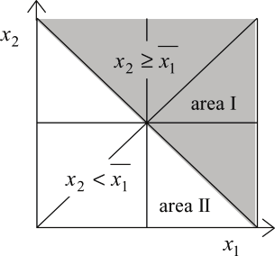
the number of the areas is 8), but not (2 n)! that is seen from the Fig. 2a, where the square
[0,1]2 partitioning is shown. In Fig. 2a the number of each area coincides with the number of
situation indicated above, for which the relations between arguments in the given situation
and values of the function f ( x , x ) = ( x ∧ x ) ∨ ( x ∧ x ) for each area are shown in the table, 1
2
1
2
1
2
presented in Fig. 2b. At all points in the same area the function value, not in case of const "0"
∨
~
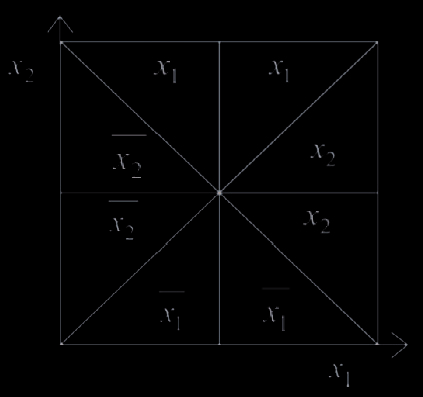
and "1", equals one of either the arguments or the complements. Fig. 2c shows values of EQ
function (notation from pap
∨
er (Krasilenko et al., 1997, a)), which is calculated in the
following way: ~
EQ ( x , x ) = x ∧ x ∨ ( x ∧ x ) . Fig. 2d shows relations between x and x 1
2
1
2
1
2
2
1
for area I (the shaded area) and area II. Fig. 2e shows pairs, setting order relations between
pairs, the connections in the pairs are shown by dotted and solid lines. Each situation of
known subcode is definitely determined by setting of order relations between pairs and the
number of such pairs equals 4 for n=2 (see Fig. 2e), in general case
2
2
n + 2 C = n . Table (Fig.
n
2b) shows the states of comparators K ÷ K signals, comparing by pair the order relations
1
4
in Fig. 2e. The usage of decoder, converting 4-digit binary codes at the output of
comparators in 8-digit one-positional code (this is the difference between our approach
from the approach, known from paper ( Shimbirev, 1990, a), and in general case n 2-digit code
of comparators into (
2 n
H = 2! )-digit one-positional code, allows by means of formation of
H adjusting signals y from the set of 2 n arranged variables { x , … x , x , … x } to h
1
n
1
n
select for each situation one of 2 n arguments (direct or i∨ts complement). I
∨ n our modified
~
~
variant, as it is seen from Fig. 2,c,d the value of EQ function ( EQ ∈{ x , x , x , x } ) 1
2
1
2
determines one of the regions {7, 2, 3, 5} in the area I or one of the regions {4, 6, 8, 1} in the
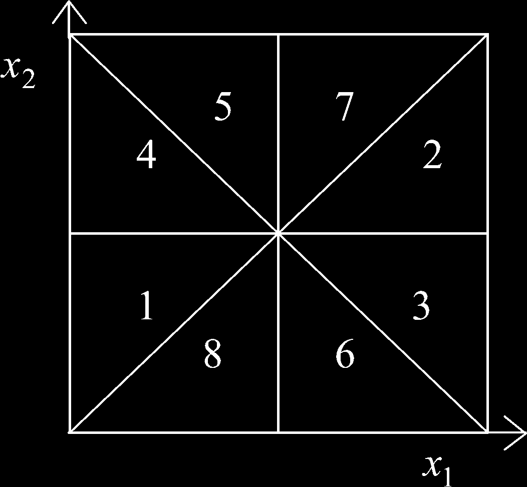
470
Optoelectronic Devices and Properties
Fig. 2a. The number of each area coincides with the number of situation indicated above, for
which the relations between arguments in the given situation and values of the function
Comparators
Region Situation
Situation f ( x , x
1
2 )
outputs
1 2 3 4
1
0 ≤ x ≤ x ≤ 1 2
x
1
2
x ≤ x ≤ x ≤ x
1 0 1 0
1
2
2
1
2
2
0 ≤ x ≤ x ≤ 0.5
x ≤ x ≤ x ≤ x
x
0 1 0 1
1
2
1
2
2
1
2
3
0 ≤ x ≤ x ≤ 0.5
x ≤ x ≤ x ≤ x
x
0 1 1 1
1
2
1
2
2
1
2
4
0 ≤ x ≤ x ≤ 0.5
x ≤ x ≤ x ≤ x
x
1 0 0 0
1
2
1
2
2
1
2
5
0 ≤ x ≤ x ≤ 0.5
≤
≤
2
1
x
≤
2
1
x
1
x
x 2
1
x
1 1 0 0
6
0 ≤ x ≤ x ≤ 0.5
≤
≤
2
1
x
≤
2
1
x
1
x
x 2
1
x
0 0 1 1
7
0 ≤ x ≤ x ≤ 0.5
≤
≤
2
1
x
≤
2
1
x
1
x
x 2
1
x
1 1 0 1
8
0 ≤ x ≤ x ≤ 5
.
0
2
1
x ≤
≤
≤
x
2
1
x
1
x
x 2
1
0 0 1 0
Fig. 2b. Table shows the states of comparators K ÷ K signals, comparing by pair the order
1
4
relations in Fig. 2e
∨
~
Fig. 2c. Values of EQ function, which is calculated in the following way:
∨
~
EQ ( x , x ) = x ∧ x ∨ ( x ∧ x )
1
2
1
2
1
2