Mechanisms, In: Advances in Robot Kinematics, 293-302, Kluwer Academic
Publishers, Dordrecht
Pott, A. (2007). Analyse und Synthese von Werkzeugmaschinen mit paralleler Kinematik,
Fortschritt-Berichte VDI, Reihe 20, Nr. 409, VDI Verlag, Düsseldorf
Pott, A.; Kecskeméthy, A.; Hiller, M. (2007). A Simplified Force-Based Method for the
Linearization and Sensitivity Analysis of Complex Manipulation Systems.
Mechanism and Machine Theory, Vol. 42, No. 11, 1445-1461
Pritschow, G.; Boye, T.; Franitza, T. (2004). Potentials and Limitations of the Linapod's Basic
Kinematic Model, Proceedings of the 4th Chemnitz Parallel Kinematics Seminar, 331-
345, Verlag Wissenschaftliche Scripten, Chemnitz
Rebeck, E. & Zhang, G. (1999). A method for evaluating the stiffness of a hexapod machine
tool support structure. International Journal of Flexible Automation and Integrated
Manufacturing, Vol. 7, 149-165
Song, J.; Mou, J.-I.; King, C. (1999). Error Modeling and Compensation for Parallel
Kinematic Machines, In: Parallel Kinematic Maschines, 172-187, Springer-Verlag,
London
Wittwer, J. W.; Chase, K. W.; Howell, L. L. (2004). The Direct Linearization Method Applied
to Position Error in Kinematic Linkages. Mechanism and Machine Theory, Vol. 39,
No. 7, 681-693
Woernle, C. (1988). Ein systematisches Verfahren zur Aufstellung der geometrischen
Schließbedingungen in kinematischen Schleifen mit Anwendung bei der
Rückwärtstransformation für Industrieroboter, Fortschritt-Berichte VDI, Reihe 18,
Nr. 18, VDI Verlag, Düsseldorf
Wurst, K.-H. (1998). Linapod – Machine Tools as Parallel Link System in a Modular Design,
Proceedings of the 1st European-American Forum on Parallel Kinematic Machines, Milan,
Italy
174
Parallel Manipulators, Towards New Applications
Zhao, J.-W.; Fan, K.-C.; Chang, T.-H.; Li, Z. (2002). Error Analysis of a Serial-Parallel Type
Machine Tool. International Journal of Advanced Manufacturing Technology, Vol. 19,
174-179
9
Certified Solving and Synthesis on Modeling of
the Kinematics. Problems of Gough-Type
Parallel Manipulators with an
Exact Algebraic Method
Luc Rolland
University of Central Lancashire
United Kingdom*
1. Introduction
The significant advantages of parallel robots over serial manipulators are now well known.
However, they still pose a serious challenge when considering their kinematics. This paper
covers the state-of-the-art on modeling issues and certified solving of kinematics problems.
Parallel manipulator architectures can be divided into two categories: planar and spatial.
Firstly, the typical planar parallel manipulator contains three kinematics chains lying on one
plane where the resulting end-effector displacements are restricted. The majority of these
mechanisms fall into the category of the 3-RPR generic planar manipulator, [Gosselin 1994,
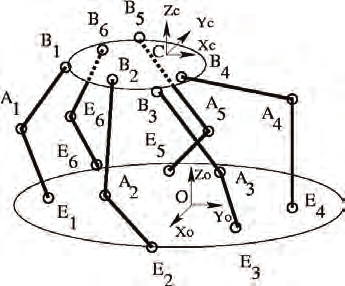
Rolland 2006]. Secondly, the typical spatial parallel manipulator is an hexapod constituted
by six kinematics chains and a sensor number corresponding to the actuator number,
namely the 6-6 general manipulator, fig. 1.
Fig. 1. The general 6-6 hexapod manipulators
Solving the FKP of general parallel manipulators was identified as finding the real roots of a
system of non-linear equations with a finite number of complex roots. For the 3-RPR, 8
assembly modes were first counted, [Primerose and Freudenstein 1969]. Hunt geometrically
demonstrated that the 3-RPR could yield 6 assembly modes, [Hunt 1983]. The numeric
176
Parallel Manipulators, Towards New Applications
iteration methods such as the very popular Newton one were first implemented,
[Dieudonne 1972, Merlet 1987, Sugimoto 1987]. They only converge on one real root and the
method can even fail to compute it. To compute all the solutions, polynomial equations
were justified, [Gosselin and Angeles 1988]. Ronga, Lazard and Mourrain have established
that the general 6-6 hexapod FKP has 40 complex solutions using respectively Gröbner
bases, Chern classes of vector bundles and explicit elimination techniques, [Ronga and Vust
1992, Lazard 1993, Mourrain 1993a]. The continuation method was then applied to find the
solutions, [Raghavan 1993], however, it will be explained why they are prone to miss some
solutions, [Rolland 2003]. Computer algebra was then selected in order to manipulate exact
intermediate results and solve the issue of numeric instabilities related to round-off errors so
common with purely numerical methods. Using variable elimination, for the 3-RPR, 6
complex solutions were calculated [Gosselin 1994] and, for the 6-6, Husty and Wampler
applied resultants to solve the FKP with success, [Husty 1996, Wampler 96]. However,
resultant or dialytic elimination can add spurious solutions, [Rolland 2003] and it will be
demonstrated how these can be hidden in the polynomial leading coefficients. Inasmuch, a
sole univariate polynomial cannot be proven equivalent to a complete system of several
polynomials. Intervals analyses were also implemented with the Newton method to certify
results, [Didrit et al. 1998, Merlet 2004]. However, these methods are often plagued by the
usual Jacobian inversion problems and thus cannot guarantee to find solutions in all non-
singular instances. The geometric iterative method has shown promises, [Petuya et al. 2005],
but, as for any other iterative methods, it needs a proper initial guess.
Hence, this justified the implementation of an exact method based on proven variable
elimination leading to an equivalent system preserving original system properties. The
proposed method uses Gröbner bases and the rational univariate representation, [Faugère
1999, Rouillier 1999, Rouillier and Zimmermann 2001], implementing specific techniques in
the specific context of the FKP, [Rolland 2005]. Three journal articles have been covering this
question for the general planar and spatial manipulators [Rolland 2005, Rolland 2006,
Rolland 2007]. This algebraic method will be fully detailed in this chapter.
This document is divided into 3 main topics distributed into five sections. The first part
describes the kinematics fundamentals and definitions upon which the exact models are
built. The second section details the two models for the inverse kinematics problem,
addresses the issue of the kinematics modeling aimed at its adequate algebraic resolution.
The third section describes the ten formulations for the forward kinematics problem. They
are classified into two families: the displacement based models and position based ones. The
fourth section gives a brief description of the theoretical information about the selected exact
algebraic method. The method implements proven variable elimination and the algorithms
compute two important mathematical objects which shall be described: a Gröbner Basis and
the Rational Univariate Representation including a univariate equation. In the fifth section,
one FKP typical example shall be solved implementing the ten identified kinematics models.
Comparing the results, three kinematics models shall be retained. The selected manipulator
is a generic 6-6 in a realistic configuration, measured on a real parallel robot prototype
constructed from a theoretically singularity-free design. Further computation trials shall be
performed on the effective 6-6 and theoretical one to improve response times and result files
sizes. Consequently, the effective configuration does not feature the geometric properties
specified on the theoretical design. Hence, the FKP of theoretical designs shall be studied
and their kinematics results compared and analyzed. Moreover, the posture analysis or
assembly mode issue shall be covered.
Certified Solving and Synthesis on Modeling of the Kinematics. Problems of Gough-Type
Parallel Manipulators with an Exact Algebraic Method
177
2. Kinematics of parallel manipulator
2.1 Kinematics notations and hypotheses
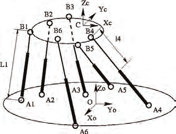
Fig. 2. Typical kinematics chains
The parallel Gough platform, namely 6-6, is constituted by six kinematics chains, fig. 2. It is
characterized by its mechanical configuration parameters and the joint variables. The
configuration parameters are thus OAR f as the base geometry and CBR m as the mobile
platform geometry. The joint variables are described as ρ the joint actuator positions
(angular or linear). Lets assume rigid kinematics chains, a rigid mobile platform, a rigid base
and frictionless ball joints between platforms and kinematics chains.
2.2 Hexapod exact modeling
Stringent applications such as milling or surgery require kinematics models as close as
possible to exactness. Realistically, any effective configuration always comprises small but
significant manufacturing errors, [Vischer 1996, Patel & Ehmann 1997]. Hence, any
constructed parallel manipulator never corresponds to the theoretical one where specific
geometric properties may have been chosen, for example, to alleviate singularities or to
simplify kinematics solving. Two prismatic actuator axes may be neither collinear nor
parallel and may not even intersect. Whilst knowing joints prone to many imperfections,
then rotation axes are not intersecting and the angles between them are never
perpendicular. Moreover, real ball joints differ from a perfectly circular shape and friction
induces unforeseeable joint shape modification, which results into unknown axis changes.
However, the joint axis angles stay almost perpendicular and any rotation combination shall
be feasible. In a similar fashion, the Cardan joint axes are not perpendicular and may be
separated by a small offset. Finally, the articulation center is not crossed by any axis.
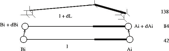
Identified the hexapode 138, the exact geometric model is then characterized by 138
configuration parameters. Each kinematics chain is described by 23 parameters, as shown on
fig. 2 and defined hereafter:
•
the 3 parameters of each base joint Ai with their error vector δ Ai ,
•
the 3 joint Ai inter-axis distances є1a , є2a and є3a
•
each prismatic joint measured position li with its error coordinate δ Li ,
•
the 3 parameters of the minimum distance between the two prismatic actuator axes: d ,
r
•
the angular deviation between the two prismatic actuator axes: φ,
•
the 3 parameters of the platform joint Bi with their error vector δ Bi,
•
the 3 joint Bi inter-axis distances and є1b, є2b and є3b
178
Parallel Manipulators, Towards New Applications
To solve this model includes the determination of parameters which cannot be measured
neither determined. Moreover, the model includes more variables than equations and
therefore, its resolution would then only be possible through optimization methods. Relying
on a calibration procedure would only determine configuration parameters by specifying an
error margin consisting of a radius around joint positions and would not indicate the
direction of the error vector. Hence, only an error ball becomes applicable to the model. In
practice, the δ Ai and δ Bi joint error vectors shall reposition the respective kinematics chains
by adding an offset to the joint centers. Thus, a random function shall compute the δ Ai and
δ Bi vectors with the maximum being the error ball radius. Finally, the selected model,
namely the hexapod 84, is effectively based on the hexapod 42 model with errors added to the
configuration data and joint variables.
2.3 Kinematics problems
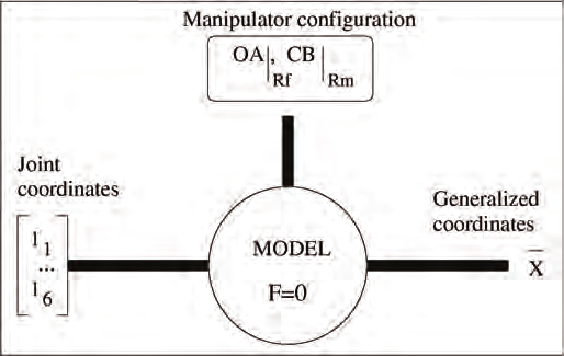
Definition 2.1 The kinematics model is an implicit relation between the configuration parameters
and the posture variables, F( X , Γ, OA|Rf, CB|Rm )=0 where Γ = {ρ 1, ρ 2,…, ρ 6}.
Fig. 3. Kinematics model
Three problems can be derived from the above relation: the forward kinematics problem
(FKP), the inverse kinematics problem (IKP) and the kinematics calibration problem, fig. 3.
The two first problems shall be covered in this article. The inverse kinematics problem (IKP)
is defined as:
Definition 2.2 Given the generalized coordinates of the manipulator end-effector, find the joint
positions.
The 6-6 IKP yields explicit solutions from vector Γ = G( X , OA|R f, CB|Rm ) and is used to prepare the FKP which is defined as:
Definition 2.3 Given the joint positions Γ , find the generalized coordinates X of the manipulator
end-effector.
The 6-6 FKP is a difficult problem, [Merlet 1994, Raghavan and Roth 1995] and explicit
solutions X = G(Γ , OA|R f , CB|Rm) have not yet been established. The difficulties in solving the FKP have hampered the application of parallel robot in the milling industry.
Certified Solving and Synthesis on Modeling of the Kinematics. Problems of Gough-Type
Parallel Manipulators with an Exact Algebraic Method
179
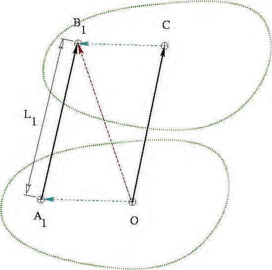
2.4 Vectorial formulation of the basic kinematics model
Fig 4. The vectorial formulation
The vectorial formulation produces an equation system which contains the same number of
equations as the number of variables, fig. (4), [Dieudonne et al. 1972]. A closed vector cycle
is constituted between the manipulator characteristic points: Ai and Bi, kinematics chain
attachment points, O the fixed base reference frame and C the mobile platform reference
frame. For each kinematics chain, a function between points Ai and Bi expresses the
generalized coordinates X, such as A B = U
A B is determined with
i
i
1( X). Inasmuch, vector
i
i
the joint coordinates Γ and X giving a function U2( X, Γ). Finally, the following equality has
to be solved: U1( X) = U2( X, Γ).
3. The inverse kinematics problem
For each kinematics chain, i = 1, ..., 6, each platform point OBi| Rf can be expressed in terms of
the distance constraint, [Merlet 1997]:
2
2 =
, i = 1...6
l
(1)
i
AiBi
Using the vectorial formulation, two equation families can be derived: displacement-based
and position-based equations.
3.1 Displacement based equations
Any mobile platform position
|
OB Rf which meets constraints 1 has a rotation matrix ℜ such
that:
|
i
OB R = OC
+ℜ⋅ CB
i = …
(2)
f
|
i Rf
|
i m
R ,
1 6
180
Parallel Manipulators, Towards New Applications
Substituting 2 in 1, we obtain:
2
2 =
| R + ℜ ⋅
−
= …
f
|
i Rm
|
i R
i
l
OC
CB
OA
i
f
,
1 6
(3)
This last equation system can be developed and simplified, leading to the IKP :
2
2
2
= ( | R −
+
−
ℜ⋅
+
f
|
i Rf )
( | Rf
|
i Rf )
|
i m
R
i
i
l
OC
OA
OC
OA
CB
CB
(4)
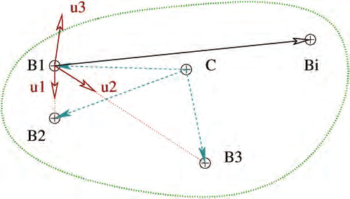
3.2 Position based equations
In 3D space, any rigid body can be positioned by 3 of its distinct non-colinear points,
[Fischer and Daniel 1992, Lazard 1992b]. The 3 mobile platform distinct points are usually
selected as the 3 joint centers B1, B2, B3, fig. 5. The 6 variables are set as: OBi| Rf = [ xi, yi, zi] for i
= 1 . . . 3. The OBi| Rf parameters define the reference frame Rb1 relative to the mobile
platform and B1 is chosen as its center. The frame axes u1, u2 and u3 are determined by the 3
platform points:
1
B B
B B
2
1 3
=
=
= ∧
1
u
, 2
u
, 3
u
1
u
2
u (5)
1
B 2
B
1
B 3
B
Any platform point M can be expressed by B M = a
1
Mu1 + bMu2 + cMu3 where aM, bM, cM are
constants in terms of these three points. Hence, in the case of the IKP, the constants are
noted aBi, bBi, cBi, i = i . . . 6 and can explicitly be deduced from CB| Rm by solving the
following linear system of equations:
B
=
+
+
= …
1 B
a u
b u
c u i
i R
B
B
B
,
1
6
|
(6)
b
i
1
i
2
i
3
1
Fig. 5. The platform three point coordinate system
Certified Solving and Synthesis on Modeling of the Kinematics. Problems of Gough-Type
Parallel Manipulators with an Exact Algebraic Method
181
Substituting relations 6 in the distance equations li2 = ║ A B
i
i | Rf║, i = 1 . . . 6, the system can
be expressed with respect to the variables xi, yi, zi , i = 1, 2, 3. Thus, for i = 1 . . . 6, the IKP is obtained by isolating the ρi or li linear actuator variables in the six following equations:
l = ( x − OA ) +( y −
i =
(7)
i
OA )2
2
2
,
1...3
i
i
ix
iy
2
2
l = B | kR − O A
i = …
(8)