Newton-Raphson-algorithm.
4. The platform updatest the KBi with μ(y*).
5. Each leg determines the dependent angles of the passive joints from the known
values of (KBi,KCi,qi).
Thus, a comprehensive algorithm for forward kinematics for the Stewart-Gough-platform,
the Delta-robot, and Linapod like machines is presented. Note, that by using the kinetostatic
methods one also receives these relations in terms of velocity, acceleration, and force. The
resulting kinetostatic model can be used for a wide range of functions for kinematic analysis
e.g. forward kinematics, calculation of the Jacobian matrix, and dexterity indexes, and
equations of motion. The discussion of all these algorithms is out of the scope of the paper.
In the following section, the determination of a geometrical linearization will be highlighted.
2.4 Linearization and sensitivity analysis
In this study, the function of the forward kinematics of a multi-body system is denoted by φ
(q, g), where q are the generalized independent joint coordinates, and g collects all geometric
parameters of the manipulator. The evaluation of the forward kinematics yields the world
coordinates y of a particular point of the end-effector of a manipulator together with the
orientation of the end-effector, which shall be denoted here as end-effector frame (EEF). For
most of the non-serial mechanisms, the function of the forward kinematics φ is not unique,
since there may be multiple positions for the EEF that correspond to a given set of
generalized joint coordinates q due to different assembly modes. Here, it is assumed that it
is possible to choose the solution that corresponds to the actual assembly mode, e.g. by
162
Parallel Manipulators, Towards New Applications
giving appropriate initial conditions. The linearization of the mechanism is formally
achieved by taking the derivative with respect to the variables q and g, respectively, i.e. as
(
∂ϕ q, g)
∂ (
ϕ ,
q g)
(
∂ϕ q, g)
δy =
δ(q, g) =
δq +
δg = J δq + J δg .
(10)
q
g
∂( ,
q g)
∂q
∂g
Here, quantities δy , δq , δg denote infinitesimal variations of the aforementioned
coordinates, while Jq denotes the well-known Jacobian matrix that is related to the kinematic
dexterity of the manipulator. The matrix Jg is also a Jacobian matrix which characterizes the
sensitivity of the position y of the EEF with respect to small changes, e.g. errors, in
geometric parameters and which is used for sensitivity analysis.
For serial manipulators with n dof, the function φ can be written analytically in terms of the
Denavit-Hartenberg-parameters (α,θ,d,a)i (Denavit & Hartenberg, 1955) and the vector of
the geometric parameters becomes
g= [α 1,θ1,d1,a1,…, α n,θn,dn,an]T.
(11)
Thus, the Jacobian matrices Jq and Jg can be calculated symbolically for serial manipulators.
For nontrivial robots, however, the expressions are usually so extensive that they only can
be handled by means of computer algebra.
Complex manipulator systems are characterized by the occurrence of closed kinematic
loops. Such mechanisms have more joints than degrees-of-freedom, and the joint
coordinates are coupled through closure conditions. This implies that the expressions for φ
are either complicated, or that φ can only be computed point-wise by the iterative solution
of an implicit system of nonlinear constraints the latter being the general case which occurs
especially for parallel kinematic mechanisms that involve multiple coupled loops. Closed
kinematic loops also occur in transmission mechanisms that can be found for instance in
hydraulically driven manipulators like excavators or large scale manipulators, since they
support the force transmission.
To overcome the lack of an analytical forward kinematic function for complex manipulators,
the loop closure conditions f(y, g)=0 can be utilized for sensitivity analysis; by applying
implicit differentiation (see e.g. Wittwer et al., 2004), one obtains
∂f(y, g)
∂f(y, g)
δy +
δg = Aδy + δ
B g = 0 .
(12)
∂y
∂g
where y=[xT, θT]T are the world coordinates of the end-effector frame, e.g. in form of a
position vector x in R³ and the orientation θ holding e.g. Bryant angles, and g are the
geometric parameters. Then, one immediately obtains for the variation of the EEF world
coordinates δy=A-1Bδg, where the matrix A-1B maps the errors δg in the components to the displacements δy of the EEF (Wittwer et al., 2004).
There are certain drawbacks to this approach: First, for mechanisms with more than three
dof, an analytical form of matrix A-1 can hardly be handled due to the length of the
corresponding expressions. Second, if sensitivity analysis is established on the closure
condition, one cannot access geometric parameters that are canceled ad-hoc through the
formulation of the closure conditions. For example, the normal distance between the joint
axes in universal joints is often eliminated because the number of closure constraints can be
significantly reduced by assuming it to be exactly zero.
Kinematic Modeling, Linearization and First-Order Error Analysis
163
2.5 Linearization of manipulator systems
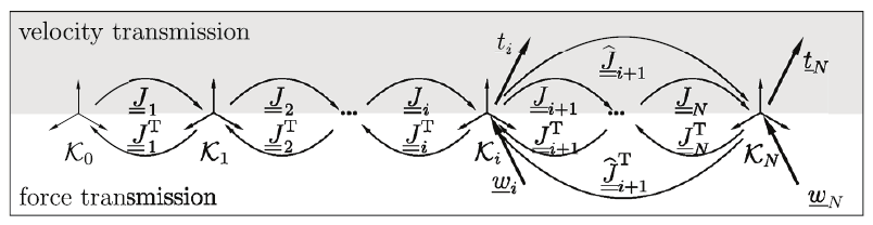
Fig. 5. Velocity and force transmission in a chain of kinetostatic transmission elements
Applying the kinetostatic formalism provides a procedure to calculate position, velocity,
acceleration, and force transmission for an arbitrary manipulator. In general, this results in a
chain of transmission elements as depicted in Fig. 5, where the individual mapping can also
correspond to closed kinematic loops since such loops are also represented by transmission
elements. In this figure, a twist T
T
T
t = ⎡ω , v ⎤ denotes the combination of an angular velocity
i
i
i
⎣
⎦
ωi of a frame K i and its corresponding velocity vi of its origin, both decomposed in some
frame. A wrench T
T
T
w = ⎡m , f ⎤ is composed of an applied moment m
i
i
i
⎣
⎦
i at the frame K i and
an applied force fi at its origin, again decomposed in some frame. Given a certain set of joint
coordinates q, one can introduce a virtual twist displacement T
T
T
δt = ⎡δφ ,δr ⎤ at the frame
i
i
i
⎣
⎦
K i, where δri is a virtual translational displacement and δφi is an infinitesimal rotational
increment in the space of rigid-body rotations, and study the corresponding virtual twist
displacement δtN at the EEF K N. This linear relation is given by
ˆ
δt = J J ... J δt = J δt ,
(13)
N
( i+1 i+2 N ) i i 1+ i
where Ji denotes the Jacobian of the velocity transmission from frame K i-1 to the frame K i.
Using kinematical differentials (Sec. 2.2) one calculates the Jacobian ˆJ , which contains the
i+1
sensitivity of the frame K N with respect to displacements in K i, and then concatenates the
matrices ˆT
J for the sought matrix T
J = ⎡ˆT ˆT
ˆT
J , J ,..., ⎤
J
. Thus, for a comprehensive
i
g
1
2
N
⎣
⎦
linearization, one needs six passes of the velocity transmission function for each ˆT
J and
i
hence 6N passes for the whole manipulator.
In contrast, one can evaluate the force transmission function, relating the wrench wN at the
EEF to the internal wrenches T
T
T
w = ⎡m , f ⎤ at the intermediate frames K
i
i
i
⎣
⎦
i, where mi
represents the moment being applied to the frame K i from the base-distal subchain to the
base-proximal subchain, and fi is the corresponding force with respect to the origin. Due to
kinetostatic duality, one obtains
w = (J J ... J
w = J w .
(14)
+
+
)T
ˆT
i
i 1 i 2
N
N
i+1
N
The force transmission presents the major advantage that one can use w
î+1 to determine J .
i
Therefore, only 6 passes of the force transmission are needed to calculate the complete
164
Parallel Manipulators, Towards New Applications
Jacobian Jg. This leads to the following simple algorithm to determine the sensitivity
Jacobian Jg:
1. Solve the forward kinematics for the desired set of joint coordinates q of the
manipulator
2. Choose unit forces Fx, Fy , Fz and unit torques Mx, My, Mz with
|Fx|=|Fy|=…=|Mz|=1 along the axes x, y, z of the EEF, respectively.
3. For each of the unit loads described above, perform the following steps:
a) Apply the load to the EEF and compute the internal forces/torques wi for each
internal frame K i one is interested in.
b) Store the internal forces/torques wi in the respective row of the Jacobian Jg.
a)
b)
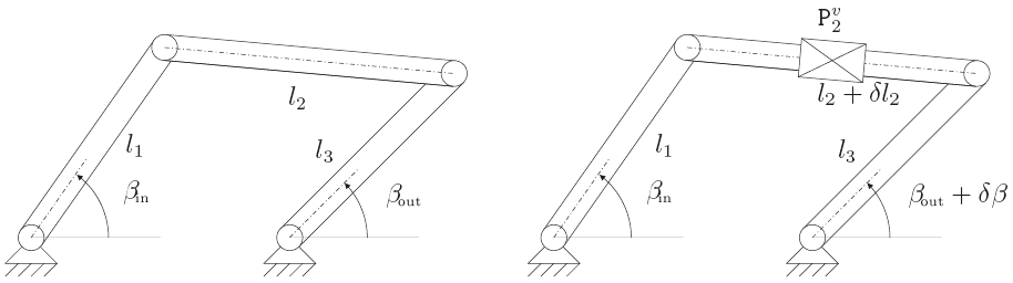
Fig. 6. Planar four-bar mechanism a) with nominal geometry b) with virtual error joint for
changes δl2 in length l2 of the coupler
2.6 Virtual error joints
The relations in the previous section can be intuitively illustrated by virtual error joints which
were introduced by Woernle (1988) and extended by Pott and Hiller (2004). The basic idea is
to insert additional independent joints which allow motion in the direction of the expected
errors. Fig. 6a presents a mechanism that involves a kinematic loop. For this planar four-bar
mechanism, one might wish to investigate the influence of changes in length of the coupler.
One introduces an additional prismatic joint in which the variation of the length of the
coupler is embodied (Fig. 6b) and the influence of changes in length of the coupler can be
calculated by using the velocity transmission. The algorithm in Sec. 2.5 can also be derived
using this model (Pott & Hiller, 2004), where the virtual error joints are used to measure the
back-propagated forces.
Based on the linearization algorithm described above, a number of applications can be
investigated, as described next.
3. Applications
3.1 Manufacturing error analysis
The Jacobian matrix Jg permits to study the influence of geometric errors on the accuracy of
the EEF. These errors may arise from the manufacturing and assembly process of the
manipulator. They cannot be avoided, but may be controlled through more precise, but at
the same time more expensive manufacturing techniques. Consequently, a comprehensive
analysis of the influence of changes in parameters is useful for optimal system design. This
analysis is basically done evaluating the Jacobian Jg mapping parameter variations δg to the
Kinematic Modeling, Linearization and First-Order Error Analysis
165
displacement δy of the EEF. The magnitude of geometric errors δgi is normally small
compared to the nominal parameter δgi. Therefore, the error estimated by the linear model
is very close to the error calculated with the generally nonlinear model (Sec. 4.2).
For different manipulators of the same type, the actual kinematic parameters may vary
within the tolerance intervals defined by the manufacturing and assembly process. Here, it
is assumed that the actual errors are Gaussian variables with a standard deviation
proportional to the tolerance. The changes in parameters are assumed to be small and
independent. Thus, the square of the total error is equal to the sum of squares of the single
errors obtained by propagation of the manufacturing, clearance, and assembly errors.
For the addition of two Gaussian variables, the standard variation of the sum becomes
2
2
σ = σ + σ , where σ
1
2
1, σ2 denote the standard deviations of each summand. In the case of a
three-dimensional vector, the total error becomes
2
2
2
2
e
Δ = e + e + e , where e
x
y
z
x,ey,ez are the
errors in the three components. For the columns of the Jacobian, one has to mix rotational
and translational components. This requires the introduction of metric coefficients that
relate rotations to translations and vice versa. Such metric coefficients can be regarded as
virtual levers that map rotations at one end to translations at the other and thus generate
sensitivities such as “long and slender” (orientations over-emphasized) or “short and thick”
(rotations under-emphasized). Assuming that standard deviations σi are known for all
geometric parameters, the error of the EEF becomes
2
Δe = ∑∑(ρ [J ] σ ) .
(15)
k
g ik
i
i
k
where [Jg]ik denote the entries of the Jacobian and ρk are the aforementioned metric
coefficients. For the case of an identical standard deviation σ for all components σi one
obtains
2
Δe = σ ∑∑[J ] = σˆσ .
(16)
g ik
i
k
Here, ˆσ is referred to as the overall error amplification index since it estimates the sensitivity of
the whole manipulator at a given configuration with respect to geometric errors. This index
is similar to the statistical approach to error analysis of Wittwer et al. (2004).
If a certain accuracy is required for a specific task, the maximal error Δemax of the EEF is
known and one can estimate the average standard deviation σ= Δemax/ ˆσ that is needed for
the geometric parameters. This is illustrated in example Sec. 4.2.
3.2 Stiffness analysis
The linearization of a manipulator with respect to its geometric parameters provides a linear
mapping between infinitesimal changes in the geometry and infinitesimal variations of the
EEF. Assume Jg to be the Jacobian transmitting infinitesimal twists δti at each of the frames
K i to infinitesimal twists δtEEF at the end-effector frame K EEF. Moreover, denote by δwEEF a small wrench being applied to the end-effector frame K EEF and by δwi the corresponding
wrenches at the frames K i ensuring static equilibrium. The Jacobian Jg can be used to set up
the stiffness matrix of the mechanism as follows. As pointed out in section 2.2, by
equivalence of virtual work it holds
T
T
δw δt = δw δt
.
(17)
g
g
EEF
EEF
166
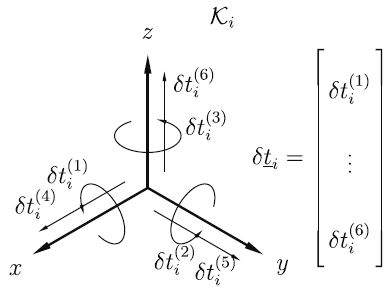
Parallel Manipulators, Towards New Applications
where δtg=[δt1,1, δt1,2,…,δtN,6]T collects all virtual variations of the geometric parameters and
δwg =[δw1,1, δw1,2,…,δwN,6]T are the respective internal forces. Here, each δti is decomposed
in its six elementary components δti,1,…,δti,6, where δti,1, δti,2, δti,3 are elementary
infinitesimal rotations and δti,4, δti,5, δti,6 are elementary translations with respect to the
coordinate frame axis (Fig. 7). Similarly, the wrench δwi =[δwi,1,…,δwi,6]T is set up.
Assuming that each elementary infinitesimal twist component δti,j produces a
corresponding infinitesimal wrench component δwi,1 by means of an associated linear
spring with stiffness coefficient ki,j, one obtains
⎧
⎫
−
⎪ 1
1
1 ⎪
−1
T
K δw = δt with
1
K = diag ⎨
,
,...,
.
(18)
g
g
g
g
⎬
⎪ k
k
k
⎩ 1,1 1,2
N,6 ⎪
⎭
Fig. 7. Decomposition of the unit twist δti at frame K i
Note that this assumption is a simplification of the structural properties of a general
mechanical component that applies to many technical applications (slender bars, joints, etc.).
The generalization to a full generic model is accomplished by a stiffness matrix in which all
coefficients may be non-zero and which may be obtained from finite element analysis. This
generalization is not further pursued here as is bears no new insight and is not required for
the examples treated in this paper. A generalization is conceivable as a later step. On the
other hand, it holds
−1
K δw
= δt .
(19)
EEF
EEF
EEF
where KEEF is the sought stiffness matrix at the EEF. Substituting Eq. (18) and Eq. (19) into
Eq. (17) and using the global force transmission
T
δw = J = δw
gives
g
g
EEF
T
1
−
T
T
1
−
δw J K J δw
= δw K δw
.
(20)
EEF g
g
g
EEF
EEF
EEF
EEF
Since this equation holds for any δwEEF, it follows
−1
1
−
T
K
= J K J .
(21)
EEF
g
g
g
Thus, the Jacobian Jg can be used to transform the stiffness coefficients ki,j of the geometric
parameters contained in the stiffness matrix Kg to the global stiffness matrix KEEF.
Kinematic Modeling, Linearization and First-Order Error Analysis
167
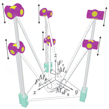
4. Examples
In this section, the proposed linearization technique is applied to analyze a six-dof parallel
kinematic machine where no closed-form solution for the forward kinematics is possible.
4.1 Error analysis for a parallel kinematic manipulator
This example considers the six-dof parallel kinematic machine tool Linapod (Pritschow et al.
2004; Wurst, 1998) installed at the Institute for Control Engineering of Machine Tools and
Manufacturing Units at the University Stuttgart (Germany), see Fig. 8. Six rigid links
connect the mobile platform to the fixed fr