b
0
0
0
0
⎞
⎜
⎟
⎜ a
a
0
b
b
0
1
0
1
0
⎟
⎜
⎟
⎜
⎟
(39)
M = ⎜ a
a
b
b
l
1
m
1 ⎟
⎜
⎟
⎜ 0 a
a
0
b
b
l
2
m
2 ⎟
⎜
⎟
⎜
⎟
⎝ 0
a
0
b
l
1 ⎠
Inasmuch, we can write: Res( P, R, x 1) = det( Sylv( P, R, x 1). If we examine the Sylvester matrix, we can observe that part with the ai parameters contains m columns and the one with bi n
columns.The following proposition holds and its proof is described in [Cox et al. 1992]: The
resultant Res( f, g, x) is the first ideal of elimination < f, g > ∩ k[ x2,…,xn] ; moreover, Res( f, g, x) = 0
iff f, g have a common factor in k[ x1,…,xn] which has a positive degree in x. The nature of this
factor has to be determined and we wish to establish if it is only one root of functions f and
g. To answer that question, the following corollary will be employed: If f, g ∈ C[ X] then Res( f, g, x) = 0 iff f and g contain a common root in C. This common root is determined by computing
det( Sylv( P, R, x 1) = 0. The nature of this root has to be determined, notably if it is a partial one and the answer will come from the following proposition, [Cox et al. 1992] : Knowing
that f, g ∈ C[ X] , let a0, b0 ≠ 0 and a0, b0 ∈ C[ x2,…, xn] , if Res( f, g, x) ∈ C[ x2,…,xn] cancels at ( c2,…,cn) , then we obtain that either a0 b0 = 0 at ( c2,…,cn) or either ∃ c1 ∈ C such as f and g cancel.
In certain instances, the head terms of the polynomials can cancel which will result in the
cancellation of the determinant and the process consequently adds one extraneous root.
In order to obtain the univariate equation, a recursive algorithm will be applied. Firstly, we
calculate n − 1 resultants hk = Res( fk+1, f 1, x 1) on variable x 1 for k = 1,…, n − 1. Secondly, we compute n − 2 resultants h(2)j = Res( hj+1, h 1, x 2) on variable x 2 for j = 1,…, n − 2 and we continue in the same fashion until the univariate equation is determined. An almost
triangular equation system is constructed.
⎡ f
…
1 ( X ) =
,
0
, f
X
,
0 f
X
,
0 f X
0
n−2 (
) =
n−1 (
) =
n (
) =
⎢ h
…
…
…
…
1 ( x ,
, x , , h
x , , x , h
x , , x
2
n )
n−2 ( 2
n )
n−1 ( 2
n )
⎢
(2)
⎢ h
…
…
…
(40)
1
( x , , x , , h 2 x , , x
3
n )
( )
n−2 ( 3
n )
⎢⎢⎢ n− h 21(
n
x , x , h 2 x , x
n−1
n )
( − )
2
( n−1 n)
⎢⎢⎣ H( xn)
The last H( xn) is the targeted univariate equation. However, this equation cannot be
considered equivalent to the initial algebraic system because the head terms can cancel.
The return step to original variables is performed by substituting back through the
triangular system. The equation is solved H( xn) = 0 and we obtain a series of w roots { xn}. We
take the w roots, one by one, which is introduced in one of the equations h 1(n−2) ( xn−1) = 0 or
h 2( n−2) ( xn−1) = 0 and obtain the w roots { xn−1}. We continue until x 1 is isolated.
The 6-6 FKP has been solved applying resultants, [Husty 1996], in a computer algebra
environment to avoid intermediate result truncation, since, in a sense, parameter truncation
can be envisioned as changing the manipulator configuration.
Certified Solving and Synthesis on Modeling of the Kinematics. Problems of Gough-Type
Parallel Manipulators with an Exact Algebraic Method
191
A variation to the resultant method is called the dialytic elimination. Let the variable set be
X = { x 1,…, xn} of the algebraic system F( X) = 0; then select any variable xi and set it as the hidden variable, then a monomial vector is constructed around xi for the system F( X) which
is expressed as W = (1, xi, xi 2,…). The FKP is rewritten as a linear system in terms of W :
W
A
= 0
(41)
where : W ≠ 0
Being a generalization of Res( P, Q, x 1) = det( Sylv( P, Q, x 1), it is subjected to the same risks of root addition through the head term cancellation. Dialytic elimination has been
implemented to solve the FKP of the 3-RS or MSSM parallel manipulators, [Griffis and
Duffy 1989, Dedieu and Norton 1990, Innocenti and Parenti-Castelli 1990]. Satisfactory
results were produced on simple parallel manipulators, [Raghavan and Roth 1995].
5.6 Gröbner Bases
Lets denote by Q[ x 1,…, xn] the ring of polynomials with rational coefficients. For any n-uple
μ = (μ
μ
μ
1,…, μn) ∈ N n, lets denote by Xμ the monomial X 1 1 ·...· X n n . If < is an admissible monomial ordering and
r
( i )
P = ∑ a X μ any polynomial in Q[ X 1,..., Xn], the following
i =
i
0
polynomial notations are necessary :
-
LM( P,<) = max i=0…r , < Xμ( i) is the leading monomial of P for the order <,
-
LC( P,<) = ai with i such that LT( P) = Xμ( i) is the leading coefficient of P for <,
-
LT( P,<) = LC( P,<)· LM( P,<) is the leading term of P for <.
Lets denote by x 1,…, x n the unknowns and S = { P 1 =,…, Ps} any polynomial system as a subset of Q[ x 1,…, x n]. A point α ∈ C n is a zero of S if Pi(α) = 0 ∀ i = 1… s. Actually, any large polynomial equation system cannot be directly or explicitly solved. Thus, it is necessary to
revert to mathematical objects containing sufficient information for resolution. Any
polynomial system is then described by an ideal:
Definition 5.5 [Cox et al. 1992] An ideal I is defined as the set of all polynomial P(X) that can be
constructed by multiplying and adding all polynomials in the ring of polynomials with the original
polynomials in the set S.
A Gröbner Basis G is then as a computable polynomial generator set of a selected polynomial
set S = { P 1,…, Ps} with good algorithmic properties and defined with respect to a monomial
ordering. This basis is a mathematical object including the ideal I information. The
lexicographic and degree reverse lexicographic ( DRL) orders are usually implemented, [Cox et
al. 1992, Geddes et al. 1994]. Given any admissible monomial ordering, the classical
Euclidean division can be extended to reduce a polynomial by another one in Q[ X 1,…, X n].
This polynomial reduction can be generalized to the reduction by a polynomial list. The
reduction output depends on the monomial ordering < and the polynomial order.
Definition 5.6 Given any admissible monomial ordering, <, a Gröbner Basis G with respect to < of
an ideal I ⊂ Q[X1,…,Xn] is a finite subset of I such that: ∀ f ∈ I , ∃ g ∈ G such that LM(g,<) divides LM(f,<).
Some useful Gröbner Basis properties are described in the following theorem:
Theorem 5.1 Let G be a Gröbner Basis G of an ideal I ⊂ Q[X1,…,Xn] for any < monomial ordering,
then a polynomial p ∈ Q[X1,…,Xn] belongs to I if and only if the reduction algorithm Reduce (p, G,<
) = 0; the reduction does not depend on the order of the polynomials in the list of G; it can be used as a
simplification function.
192
Parallel Manipulators, Towards New Applications
The classical method for computing a Gröbner Basis is based on Buchberger's algorithm
[Buchberger et al. 1982, Buchberger 1985]. Recently, Faugère proposed more powerful
algorithms, namely accel and F4 implemented in the FGb software, [Faugère 1999].
5.7 Gröbner Bases and zero dimensional systems
Definition 5.7 [ Lazard 1992a] A zero-dimensional system is defined as a mathematical equation
system with a variety (solution set) constituted by a finite number of complex points.
From a mathematical point of view, any variety is a valid result. From an engineering one,
we seek a variety which represents an exploitable result. For any parallel manipulator FKP,
the zero-dimensional systems allow pose analysis, since each real solution corresponds to each
manipulator pose. Otherwise the problems fall in the category of rarely usable singular
configurations. Detection of zero-dimensional systems is performed by implementing the
following theorem:
Theorem 5.2 Let G = {g1,…,gl} be a Gröbner Basis for any ordering < of any system S = {P1,…, Ps}
∈ Q[X1,…,Xn]s. The two following properties are equivalent:
-
For all index i, i = 1…n, there exists a polynomial gj ∈ G and a positive integer nj such that
Xinj = LM(gj,<);
-
The system {P1 = 0,…,Ps = 0} has a finite number of solutions in Cn.
Hence, one can determine if the FKP resolution yields a finite or infinite number of
solutions. This is obviously an important issue, since an algebraic system with an infinite
number of solutions (variety of degree one or higher) cannot be directly exploited by a
control system and failure is usually the outcome.
5.8 The lexicographic Gröbner Basis
The choice of the monomial ordering is critical for the Gröbner Basis computation efficiency,
which is evaluated by the computation times, the size and the shape of the result. A
lexicographic Gröbner Basis with X 1 < X 2 < … < Xn as variable order has always the following
general shape:
⎧ f X
f X X
…
1 (
1 ) =
,
0 2 ( ,1 2 ) = ,
0
⎪
f ( X , X
f
X X X
…
k
1
2 ) =
,
0 k +1( ,
,
1
2
3 )
⎪
= ,
0
(42)
⎨ 2
2
f
X … X
…
k
+1 (
,
,
1
n )
⎪
= ,
0
n−1
⎪ f X … X
k (
,
,
1
n )
⎩
= 0
n
Whilst computing a lexicographic Gröbner Basis using Buchberger's algorithm yields doubly
exponential complexity in the worst case, an order change will save computation time.
Therefore, one DRL Gröbner Basis may first be computed in dn polynomial time where d is
the maximum total degree of the equations. Then, the DRL Gröbner Basis can be converted
into a lexicographic one in O( nD 3) arithmetic operations, [Faugère et al. 1991]. In the case of
any zero-dimensional system, this can be done using exclusively linear algebra techniques,
[Faugère et al. 1991].
Definition 5.8 Let S be a system constituted by the polynomials p1,…,ps ∈ Q[x1,…,xn], without
square factors. Let G = {g1,…,gl} be a Gröbner Basis computed for any ordering < on the system S. If
the univariate polynomial f(x1) is without any multiple factors, then the equation is square-free, the
first coordinates of all solutions are distinct and the solutions yield no multiple root. Then, the system
is considered in Shape Position .
Certified Solving and Synthesis on Modeling of the Kinematics. Problems of Gough-Type
Parallel Manipulators with an Exact Algebraic Method
193
If the polynomial system is in Shape Position, the Gröbner Basis has the following
simplified univariate format:
f 1( X 1) = 0, X 2 = f 2( X 1) = 0,…, Xn = f n( X 1)
(43)
In this format, the lexicographic Gröbner Basis can be computed directly using the F4
algorithm, [Faugère 1999].
5.9 The rational univariate representation
Another root representation is given by the Rational Univariate Representation, hereafter
identified Rational Univariate Representation, [Rouillier 1999]. In the particular case of systems
in Shape Position, the univariate variable is the first one in the original system ones, so that
the Rational Univariate Representation can be written in the following format:
{ h( X =
=
…
=
(44)
k )
0, X 2 h 2 ( Xk ) / 0
h ( Xk ) , , Xn hn ( Xk ) / 0
h ( Xk )
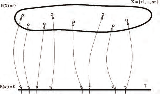
Fig. 8. The correspondence between the Rational Univariate Representation and original
system varieties.
h( Xk) where 1 ≤ k ≤ n denotes the univariate equation, hi i = 0 … n the univariate return
functions. These polynomials are elements of Q[ Xk]. Inasmuch, h and h0 are coprime.
Moreover, if the Rational Univariate Representation system is in Shape Position and if h( Xk) is
square-free, the Rational Univariate Representation can be converted into a lexicographic
Gröbner Basis and the Rational Univariate Representation expression can be simply computed
from this basis. This situation is generally the case in most FKP instantiations:
h( Xk) = f( Xk), g( Xk) = f′ ( Xk)
(45)
Moreover, since f and f 0 are coprimes, f 0 is invertible modulo f; this leads to: hi = fi ⋅ ( f′)−1
modulo f , i = 2 … n.
Definition 5.9 Let S be a system constituted by the polynomials p1,…, ps ∈ Q[x1,…,xn] and let
G = {g1,…,gl} be a Gröbner Basis for any ordering < of the system S. Then, the RR form is defined as
the system R = {p
−
−
−
−
1, p1 1p2 mod G, p1 1p3 mod G,…, p1 1pk mod G} ∈ Q[x1,…,xn] where p1 1 is
calculated such that (p1 p −
1 1 modulo G) = 1.
194
Parallel Manipulators, Towards New Applications
The rationale behind the RR form computation is to reduce the polynomial system S. The
computed Gröbner Basis G on any ordering < of the system S is used for the system
reduction. Then, the reduced system R resolution shall be less difficult.
Definition 5.10 Let S be a system constituted by the polynomials p1,…,ps ∈ Q[x1,…, xn], if the
system S is without square factors and in Shape Position and if a lexicographic Gröbner Basis is
computable, then the system RR form R′ can be deduced.
Since the S system reduction by a lexicographic Gröbner Basis leads to a further reduced
system R, one can conjecture faster FKP resolution. However, in some instances, p −
1 1 can
hardly be computed and the RR form cannot be deduced. Hence, the FKP is solved by first
computi