manipulators. Indeed, a lot of applications do not need six DOFs. A classification proposed
by Brogardh (Brogardh, 2002) gives the necessary number of DOF for different industrial
applications. He shows that applications such as pick-and-place, assembly, cutting,
measurement, etc. just need from three up to five DOFs.
The parallel manipulator H4 can provide three translations and one rotation about a fixed
axis, which are also called Schonflies motions (Herv , 1999). SCARA robots were the first
manipulators developed to produce these movements. Due their serial architecture, these
robots involve high moving masses which are not suitable for high dynamics. Parallel
architecture can overcome this problem. Delta robot is first introduced by Clavel to execute
Schonflies motions (Clavel, 1988). This architecture is able to produce three translations and
one rotational motion is obtained using a central “telescopic” leg built with universal and
prismatic joints. This RUPUR chain suffers from a short service life, and involves a bad
stiffness of the rotation motion. Orthoglide (Chablat, 2002) is another parallel robot that can
provide Schonflies motions using linear actuators. Its particularity is to be isotropic at the
center of its workspace. The machine tool HITA STT has been proposed to produce
Schonflies motions (Thurneysen et al, 2002). The particularity of this architecture is to use
additional parts in the traveling plate in order to amplify the rotational motion. Other
Schonflies motion generators include Gross Manipulator (Angeles et al., 2000), SMG
(Angeles, 2005), Kanuk and Manta (Rolland et al., 1999) robots.
In order to avoid the central telescopic leg of the Delta robot, in 1999, the Montpellier
Laboratory of Computer Science, Robotics, and Microelectronics (LIRMM) in French
invented the parallel manipulator H4 which used the concept of articulated traveling plate.
The rotational movement is obtained using an internal mobility on the traveling plate, and a
transforming device gives the desired range of rotational motion. Because placing actuators
in a symmetrical way ( i.e. at 90° one relatively to each other) involves “internal singularities”
(Pierrot & Company, 1999), the robot has to be built using a particular arrangement of
motors. This non-symmetrical arrangement entails a non-homogeneous behavior in the
workspace and a limited stiffness of the robot (Company et al., 2005). Later, based on the
concept of H4, an improved mechanical structure called I4 is proposed by LIRMM (Krut et
al., 2004; Krut et al., 2003). The internal mobility of I4 is obtained with a prismatic joint (Fig.
8). The advantage of this architecture is to authorize a symmetrical arrangement of the
actuators. As demonstrates by Krut (Krut et al., 2004), it is possible to place the actuators at
90° one relatively to each other. However, this architecture is more adapted to machine-tool
application than to high speed pick-and-place. Indeed, commercial prismatic joints are not
suitable for high speed and high accelerations, and have a short service life under such
conditions. This inconvenient is due to the high pressure exerted on the balls of these
elements at high acceleration conditions. Based on H4 and I4 architecture, an evolution of
these mechanisms, named Part 4, has been developed with the wish of reaching high speeds
414
Parallel Manipulators, Towards New Applications
and accelerations (Nabat et al., 2005). A paper written by Nabat (Nabat et al., 2006)
presented experimental results showing that Part 4 was able to reach an acceleration of 15G.
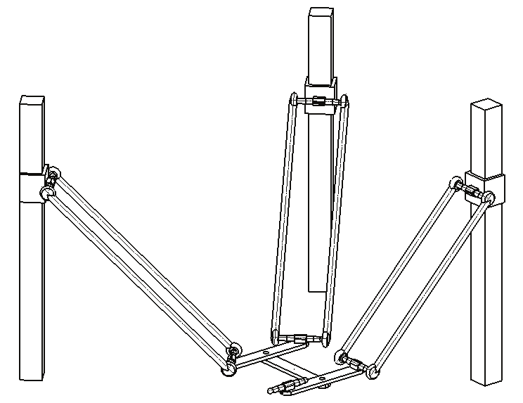
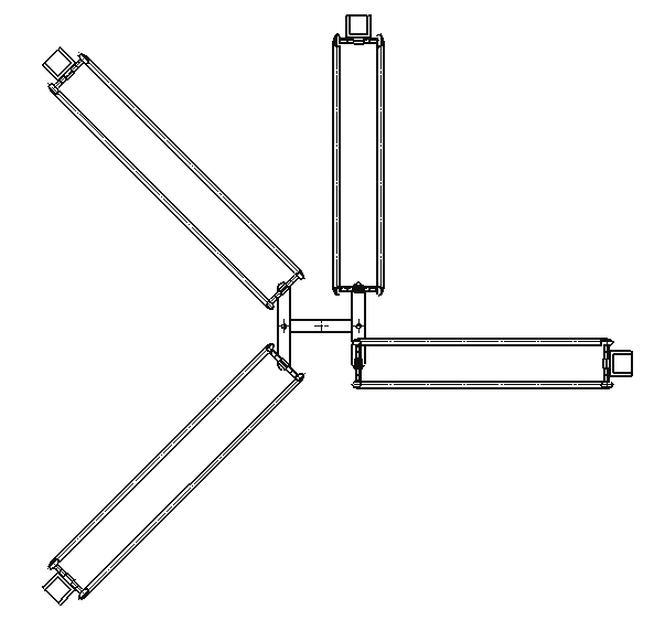
Part 4 is a parallel manipulator composed of four closed kinematic chains and an articulated
traveling plate. The kinematic chains are similar for Delta, H4 and I4, each of which is
composed of an arm and a spatial parallelogram (forearm) linked with spherical joints. The
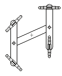
traveling plate is composed of four parts: two main parts (1, 2) linked by two bars (3, 4) with
revolute joints (see Fig.9). Thus, its shape is a planar parallelogram and the internal mobility
of this traveling plate is a circular translation. Generally, the “natural “range of the
rotational operational motion is small, in order to make a complete turn: [-π; π], an
amplification system has to be added on the traveling plate. Several options are available for
this amplification such as gears or belt/pulleys. The prototype shown in Fig.9 (b) has been
built using belt/pulleys system, with the first pulley fixed on one half traveling plate, and
the second one is linked with a revolute joint to the second half traveling plate. Due to its
traveling plate having the shape of a planar parallelogram, Part 4 has all the advantages of
the previous robots, without their drawbacks. The traveling plate of this robot is articulated
and is exclusively realized with revolute joints. Nabat (Nabat et al., 2006) has demonstrated
that it is possible to have the same arrangements of the actuators as I4. Thus, this robot is
well suited to reach high dynamics and, at the same time, to have a good stiffness and a
homogenous behavior in the workspace.
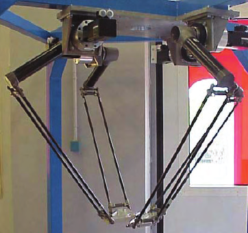
(a) Overview of I4 prototype
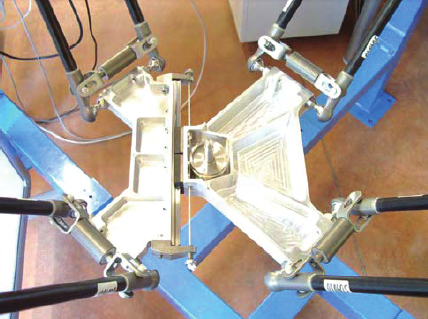
(b) Articulated traveling plate
Fig.8. I4 prototype (courtesy of LIRMM)
The use of base-mounted actuators and low-mass links allows the traveling plate to achieve
great accelerations. This makes this type of parallel manipulator a perfect candidate for pick
and place operations of light objects. Especially for semiconductor end-package equipments,
which need high-speed and high-precision pick-and-place movement, these parallel
manipulators provide a novel solution scheme.
In this chapter, only H4 is considered, because it firstly provides the most important concept
of traveling plate. Based on the analytical method of H4, other types of evolution structure
can be analyzed conveniently.
A Novel 4-DOF Parallel Manipulator H4
415
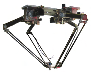
(a) Overview of Part4 prototype
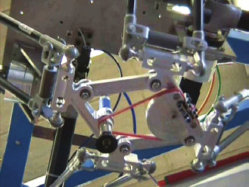
(b) Articulated traveling plate
Fig.9. Part4 prototype (courtesy of LIRMM)
3. Kinematic analysis
This section will examine the relations between the actuated joint coordinates of H4 and the
nacelle (or traveling plate) pose.
3.1 Inverse kinematics
The relation giving the actuated joint coordinates for a given pose of the end-effector is
called the inverse kinematics, which is simple for parallel robots. The inverse kinematics
consists in establishing the value of the joint coordinates corresponding to the end-effector
configuration. Establishing the inverse kinematics is essential for the position control of
parallel robots. There are multiple ways to represent the pose of a rigid body through a set
of parameters X. The most classical way is to use the coordinates in a reference frame of a
given point C of the body, and three angles to represent its orientation. But there are other
ways such as kinematic mapping which maps the displacement to a 6-dimensional
hyperquadric, the Study quadric, in a seventh-dimensional projective space. The kinematic
mapping may have an interest as equations involving displacement are algebraic (and the
structure of algebraic varieties is better understood than other non-linear structures) and
may have interesting properties, for example, stating that a point submitted to a
displacement has to lie on a given sphere is easily written as a quadric equation using Study
coordinates (Merlet, 2006).
3.1.1 Analytic method
For a fully-parallel mechanism, each of the chains link the base to the moving platform. If A
represents the end of the chain that is linked to the base, and B the end of the chain that is
linked to the moving platform. By construction the coordinates of A are known in a fixed
reference frame, while the coordinates of B may be determined from the moving platform
position and orientation. Hence the vector AB is fundamental data for the inverse kinematic
problem, this is why it plays a crucial role in the solution.
In order to write the position relationship of H4, consider the robotic structure (see Fig.10,
chain #4 is not plotted for sake of simplicity). The geometrical parameters of the
manipulator at hand are defined as follows:
416
Parallel Manipulators, Towards New Applications
•
Two frames are defined, namely {A}: a reference frame fixed on the base; {B}: a
coordinate frame fixed on the nacelle ( C 1 C 2);
•
The actuators slide along guide-ways oriented along a unitary vector, k (
z
k is the
z
unity vector along z axis in the reference frame {A}), and the origin is the point iP , so
the position of each point A is given by:
,
i
A =
+
i
i
P
qiz i q is the moving distance of the
i
actuator. The number i = ,
1
,
3
,
2 4 represents each pair of kinematic chains;
•
The parameters M d
i ,
and h are the length of the rods, the offset of the revolute-joint
from the ball-joint, and the offset of each ball-joint from the center of traveling plate,
respectively;
•
The position of the end-effector, namely point B , is defined by a position vector
B = [ x y z], and a scalar θ , representing the orientation angle.
Without losing generality, in this section we consider P = a b
for simplicity, Q is the
i
( , ,0
i
i
)
z
offset of {A} from {B} along the direction of k z .
kz
z 0
y 0
q 3
A31
A
P3
x 0
A3
A32
Q z
v1
z
y
M 3
C
1
B3
B
B
31
x
B
2 h
C
32
2
2 d
Fig.10. H4 manipulator with four lines drives and (S-S)2 chains
The position of points C1 and C2 are given by:
C = B + Rot v,θ BC
C = B + Rot v,θ BC
(7)
1
( )( 1) 2
( )( 2)
A Novel 4-DOF Parallel Manipulator H4
417
Where Rot(v,θ ) denotes the rotation matrix of nacelle with respect to reference frame. The
position of each point Bi is given by:
B = C + C B
B = C + C B
1
1
1
1
2
1
1
2
(8)
B = C + C B
B = C + C B
3
2
2
3
4
2
2
4
The position relationship can then be written as:
2
2
A B
= M
(9)
i
i
i
Then for the first axis:
A B = B + Rot v,θ BC + C B − P − q z
1 1
[
( )( 1) 1 1 1] 1 1
(A B = q − 2 q d ⋅z +d
(10)
1
1 )2
2
2
1
1 1
1
1
where d = B + Rot v,θ BC + C B − P . Finally, the two solutions are given by:
1
( )( 1) 1 1 1
q = d ⋅ z ±
d ⋅ z
+ M − d
(11)
1
1
1
( 1 1)2
2
2
1
1
Similar derivations give the solution for q 2, q 3 and q 4.
3.1.2 Geometrical method
The geometrical approach to the inverse kinematics problem is to consider that the
extremities A, B of each chain have a known position in 3D space. The leg can be cut at a
point M and two different mechanisms MA, MB constituted of the chain between A, M and
the chain between B, M can be gotten. The free motion of the joints in these two chains will
be such that point M, considered as a member of MA, will lie on a variety VA, while
considered as a member of MB it will lie on a variety VB. If assume the mechanism have only
classical lower pairs, these varieties will be algebraic with dimensions dA, dB. In the 3D
space, a variety of dimension d is defined through a set of 3- d independent equations, and
hence VA, VB will be defined by 3- dA and 3- dB equations. The solutions of the inverse
kinematic problem lie at the intersection of these varieties. As the number of of solutions
must be finite (otherwise the robot cannot be controlled), the rank of the intersection variety
must be 0. In other words, in order to determine the 3 coordinates of the points, 3- dA+3- dB
should equal to 3 or dA+ dB equal to 3 (Merlet, 2006).
The key problem about the geometrical mthod rests with the choice of the cutting point. For
the H4 structure shown in Fig.10, Bi are chosen as the cutting points. Points Bi has to lie on a
sphere centered at Ai with radius Mi, while for the nacelle, the coordinates of Points Bi can
be described as (8). Hence to obtain the intersection of these 2 varieties the known distance
between A, B of should be equal to Mi: this equation will give the joint coordinates qi. The
same results can be obtained as described as (11).
3.2 Direct kinematics
Direct kinematics addresses the problem of determining the pose of the end-effector of a
parallel manipulator from its actuated joint coordinates. This relation has a clear practical
interest for the control of the pose of the manipulator, but also for the velocity control of the
end-effector.
418
Parallel Manipulators, Towards New Applications
In general, the solutions for determining the pose of the end-effector from measurements of
the minimal set of joint coordinates that are necessary for control purposes is not unique.
There are several ways of assembling a parallel manipulator with given actuated joint
coordinates, and generally the direct kinematic relationship cannot be expressed in an
analytical manner. Although various methods have been presented for finding all the
solutions for this problem and their computation times are decreasing (Faugère, 1995;
Hesselbach & Kerle, 1995; Gosselin, 1996; Merlet, 2004), it is still difficult to use these
algorithms in a real time context. Furthermore, there is no known algorithm that allows the
determination of the current pose of the platform among the set of solutions. The numerical
methods using a-priori information on the current pose are more compatible with a real-
time context, while their convergence and robustness is an important issue. As direct
kinematics is an important issue for control, it may be necessary and interesting to
investigate how to improve the computation time. Besides the progress in algorithms and
processor speed, one possible approach to solve these problem is to add sensors (i.e. to have
more than n sensors for a n-DOF manipulator) to obtain information, allowing a faster
calculation of the current pose of the platform, at the cost of more complex hardware (Bonev
et al., 2001; Chui & Perng; 2001; Parenti-Castelli, 2001). Merlet has pointed out several
unsolved problems about the parallel robot’s direct kinematics (Merlet, 2000). Especially the
algebraic geometry and computational kinematics should bring about enough attention.
The first step of solving direct kinematics is to determine a bound on its maximal number of
solution. Then, the equations are reduced for the system to obtain the solution of a
univariate polynomial whose degree should be determined in the previous analysis. Many
researchers have tried to obtained closed-form solutions of parallel robots in a univariate
polynomial equation. Especially, the 3- and 6- DOFs parallel robots, e.g., planar, Delta,
Steward platform and Hexapod robots, have been mainly considered. This section provides
a univariate polynomial equation for H4. It is shown that the solutions of the forward
kinematics yield a 16th degree polynomial in a single variable (Choi et al., 2003).
3.2.1 Forward kinematics formulation
The forward kinematics of the H4 is the problem of computing the position and orientation
of the nacelle (traveling plate) form the motor angles or the moving distance of the actuator.
To get a closed-form solution, a univariate polynomial equation needs to be solved. The
following method is extracted from the paper written by Choi (Choi et al., 2003).
The kinematic structure of H4 is shown in Fig.10 and design parameters are shown in Fig.11.
The nacelle is composed of three parts (two lateral bars and one central bar). The four points
B
A
A
1, B 2, B 3 and B 4 form a parallelogram. Let B and A represent the homogeneous
i
i
coordinates of the points Bi in {A} and Ai in {A} respectively. Then the homogeneous
coordinates of AB and A A can be written as:
i
i
⎡
x + hE cosθ
⎤ ⎡ Pi + x ⎤
i
1
i x
⎢
⎥ ⎢
⎥
+
θ +
+ +
y hE sin
dE
Pi
y Q
A
i
1
2 i
i y
i
B
⎢
⎥ ⎢
⎥
=
=
(12)
i
⎢
z
⎥ ⎢
z
⎥
⎢
⎥ ⎢
⎥
⎣
1
⎦ ⎣
1
⎦
A A = a
b
q
1
i
[ i i
] T
i
A Novel 4-DOF Parallel Manipulator H4
419
where
i = cosθ , i = sinθ , P = hE , Q = dE , E = E = 1
− , E = E = 1, E = E = 1
− ,
x
y
i