given by:
⎡ f 1 ⎤
⎢
⎥
⎢ f 2 ⎥
−1 ⎡ e
F ⎤ ⎢ f ⎥
J
=
(52)
S
⎢
⎥ ⎢ 3 ⎥
⎣M e ⎦ ⎢ f 4 ⎥
⎢
⎥
m
⎢ C 1 ⎥
⎢⎣ mC 2 ⎥⎦
Investigating the transformation matrix J given in equation (52), one can analyze the
S
singularity of the parallel part. The columns of J are lines lying on the Klein quadric
4
M , as
S
2
they satisfy Klein’s equation (Hunt, 1978):
l l + l l + l l = 0 (53)
1 4
2 5
3 6
where each column of equation (53) is represented by its Plücker line coordinates given by
( l , l , l , l , l
.
1
2
3
4
5 , 6 ) T
l
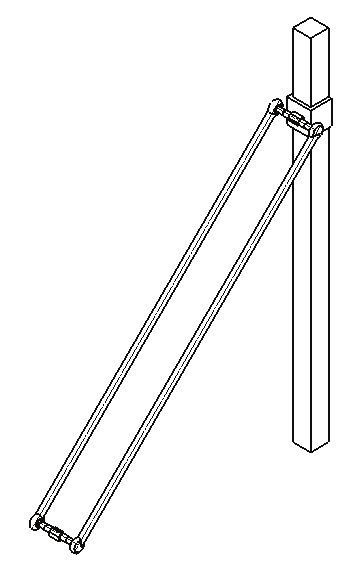
Moreover, considering the forces and moments exerted on the actuator, one can obtain (see
Fig.16).
τ
+σ
(54.1)
i k
=
z
i k pi
fiS i
f cosθ = τ
(54.2)
i
i
i
f sinθ = σ
(54.3)
i
i
i
cosθ =
(54.4)
i
k ⋅
z S i
where k is the unit vector along the direction (k ×
. Equation (54.2) can be written for
z
u i )
pi
i=1,2,3,4, and the results grouped in a matrix form, τ i can be written as:
⎡ f
τ
1 ⎤
⎡ 1 ⎤
⎢ ⎥ ⎢ ⎥
⎢ f
τ
2 ⎥
⎢ 2 ⎥
J
=
(55)
P ⎢ f ⎥ ⎢τ ⎥
⎢ 3 ⎥ ⎢ 3 ⎥
⎣ f
τ
4 ⎦
⎣ 4 ⎦
A Novel 4-DOF Parallel Manipulator H4
435
where
⎡cosθ1
0
0
0 ⎤
⎢
⎥
⎢ 0
cosθ 2
0
0 ⎥
J =
(56)
P
⎢ 0
0
cosθ
0 ⎥
⎢
3
⎥
⎣ 0
0
0
cosθ 4 ⎦
τ i
k z
A i 1
k pi
σ i
S ni
A i 2
mi
θ i
mi
B i 1
-S ni
B i 2
-S i
fi
Fig.16. Parallelogram static analysis
J (equation (52)) and
S
J (equation (56)) provide the information about the singularities of
P
the H4 manipulator. The analysis of J S provides the singularity of the parallel part of H4
robot known as the “parallel singularity” and J provides the singularity due to the
P
parallelogram structure, known as the “serial singularity”. In (Liu et al., 2003), the
singularity caused by J is also called as “actuator singularity”.
P
436
Parallel Manipulators, Towards New Applications
B i
S
A
i
i
θ i
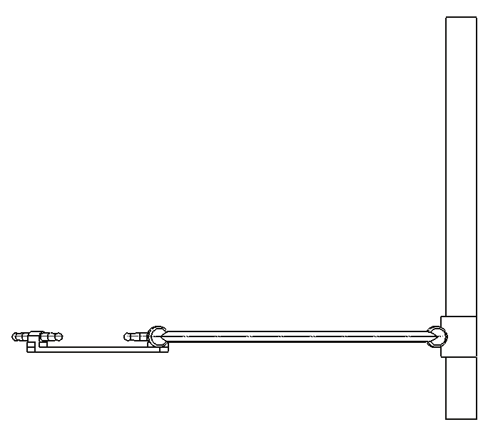
Fig.17. Serial singularity of H4 manipulator
Observing J one can see that singularity occurs whenever θ = π 2 +π ( k=1,…,n,
P
k
i
i=1,2,3,4). In this case one or more columns of J are zero and the nacelle can’t move in the
P
S direction, namely, the manipulator losses a DOF. Fig.17 shows the serial singularity of
i
H4 manipulator.
4.3 The behavior of the H4 manipulator in parallel singular configurations
The parallel singular configurations of the H4 are identified by investigating matrix J . The
S
first four columns of J define the four internal forces of parallelogram which are along the
S
direction B
(see Fig.53 and 55). Utilizing Grassmann geometry, we can obtain all
i A i
singularities of J .
S
Based on H4’s kinematic architecture, the first four columns of J can form only the
S
following linear varieties:
•
Type I: a line bundle where all lines intersect a common point, but they are not
coplanar. This is the condition 3c described in section 4.1.2.
•
Type II: all the lines belong to the union of two planar pencils of non coplanar lines that
have a line in common. This is the condition 3b described in section 4.1.2.
Type I can be considered as the special condition of Type II. When the first four columns of
J are linear dependent, the actuators can’t control the linear velocity of the nacelle,
S
generally known as “architecture singularity” (Joshi & Tsai, 2002).
The last two columns of J define the two moments of constraint which are along the
S
direction S . We make here the assumption that the two revolute joints placed on the
Ci
nacelle have the same direction represented by vector v . This choice may be not the only
one, but it worth noting that placing two revolute joints parallel to each other on the nacelle
A Novel 4-DOF Parallel Manipulator H4
437
is a good choice for practical matters. The existence of a rotational motion about v can be
written as follows (Pierrot & Company, 1999):
S
×S
≠ 0 (57)
C 1
C 2
When S ×S
= 0 , the vectors
C 1
C 2
S and
C 1
S
are linearly dependent. The constraint
C 2
moments exerted on the nacelle are along the same direction, and the robot would gain
additional DOF(s). This singularity arises from deficiency of constraints, so we call this
singularity as “constraint singularity”.
In order to investigate the instantaneous motion the robot tends to perform while in singular
configurations, the LCAA which was presented at (Pottmann et al., 1999) and further used
for robotic analysis in (Wolf & Shoham, 2003) is adopted. The LCAA is based on
determining the linear complex C = (c, c), which is the closest one to the given set of lines
L =
. The moment of
i
(l i, l i )
L with respect to a linear complex C is given by:
i
c ⋅ l + c ⋅ l
m(
i
i
L, C) =
(58)
c
Hence, given a set of lines L , the closest linear complex among all linear complexes χ can
i
be given by the minimization of:
k
∑ m(L
(59)
i , χ )
i=1
where χ is given by χ = (x x)
6
, ∈ℜ .
Equation (59) is equivalent to minimizing the positive semi-definite quadratic form given by
(Pottmann et al., 1999):
k
F(X = ∑(x⋅l + x⋅ 2
)
(60)
i
l ) = T
i
χ Mχ
i=1
D = diag(
,
1
,
1
,
1
0
,
0
,
0
)
under the normalization condition = x 2
1
χ T
=
Dχ , where
, χ presents the
χ = ( ,
x x)
6
set of all linear complexes given by
∈ℜ , and M is the Gramian matrix of J S .
Equation (60) is a general eigenvalue problem and the solution, C , is the eigenvector χ i
corresponding to the smallest eigenvalue. Moreover, given the closest linear complex found
by the algorithm, the axis, A , of the linear complex and its pitch can also be revealed. In
fact, the minimization procedure shown in above minimizes the work of the wrench applied
on the moving platform and the twists. When the smallest eigenvalue is zero, there is no
work generated by the set of wrenches when the platform moves in the twist direction given
by χ . So we can use LCAA to investigate the behavior of H4 manipulator in singular
configurations.
4.4 Simulation and results
In this section, the parallel singularities of an example H4 manipulator are presented and
the LCAA method is used to investigate the instantaneous motion the manipulator tends to
438
Parallel Manipulators, Towards New Applications
perform while in these singular configurations. For simulation, the design parameters we
have selected is described in Fig.11, where the parameters have been chosen as described in
section 3.2.2.
Architecture singularities
Architecture singular configurations of the H4 manipulator are identified using line
geometry (Merlet, 2006). Note the first four columns of J as:
S
⎡
S
S
S
S
⎤ ⎡ a
a
a
a ⎤
1
2
3
4
1
2
3
4
=
=
(61)
⎢ B
B
B
B
⎥ ⎢
⎥ [A
A
A
A
1
2
3
4 ]
R l × S
R l × S
R l × S
R l × S
⎣
a
a
a
a
D 1
1
D 1
2
D 2
3
D 2
4 ⎦
⎣ 1
2
3
4 ⎦
where a = 1 and a ⋅ a = 0 , so the six coordinates with ( a , a are called the normalized i
i )
i
i
i
Plücker coordinates of A ( i=1,2,3,4). Deriving from the geometric conditions (Type I and
i
Type II) in section 4.3, we can find that when the coordinates of point D satisfy the following
condition:
x = − 5812
.
9
y = − 4130
.
9
(62)
θ = − 5080
.
1
singularity occurs. The closest linear complex’s axis found by the algorithm is:
A = [0 0 1 −5.2937 −0.3331 0]
λ
The standard deviation of the lines form C is given by: σ =
i
= 0 , and the linear
k − 5
complex’s pitch is given by:
c ⋅
p =
c = − 4047
.
9
. Fig.18 demonstrated the result of the LCAA.
2
c
-13
-12
50
40
-11
30
-10
z 20
x
LCA
LCA
-9
10
0
-8
-50
50
-7
0
0
-6
50
-50
y
-20
-15
-10
-5
0
x
y
(a)
(b)
Fig.18. H4 robot with linear complexes (a): 3D view (b): top view
Corresponding to the non-zero pitch value of the linear complex, at this singularity the
robot performs a screw motion of rotation and translation around the linear complex axis
A .
A Novel 4-DOF Parallel Manipulator H4
439
Constraint singularities
From the discussion in section 4.3, we know that when S ×S
= 0 , the robot is in a
C 1
C 2
constraint singular configuration. If we select the structure parameters as Fig.11, when:
x = 3
− 6683
.
y = 3.3709
(63)
θ = 2
− 3905
.
the robot reaches singular configuration.
Constraint singularity occurs in limited-DOF manipulator when the screw system, formed
by the constraint wrenches in all chains, loses rank. In this section, the geometric
explanation of constraint singularity is given, then LCAA is applied to investigate the
behavior of H4 manipulator in constraint singular configuration. From the viewpoint in
(Zlatanov et al., 2002), the system of the constraining wrenches of H4, W, contains as a
subspace the 2-system of all pure moments. Then its reciprocal system, the freedoms system
T, must contain 3 translations and 1 rotation. In a H4 manipulator, the two “meta-chain”
constrain system W p contains two pure moments, one’s direction is along S , and the
C 1
other’s direction is along S C 2 . When the two moments of the two “meta-chain” are linearly
independent, two pure moments will be in W.
However, in the constraint singular configuration, S and
C 1
S
are parallel. The
C 2
constraining moments of two “meta-chain” are identical and the system W p are the same
one-system. Then, W consists of only one screw. Hence, the twist system of the robot is a
five-system and the mechanism gains new additional freedom. Applying the method of the
closest linear complex on the H4 robot in its constraint singular configuration, we can find
the closest linear complex’s axis is: A = [0.9137 0.3524 −0 2024
.
0.3208 −0 2064
.
1.0887]
and the linear complex’s pitch is:
c ⋅
p =
c =1 0469
.
. S
= −S
=
−
means
C 1
C 2
[0 3599
.
9330
.
0
0] T
2
c
that this configuration is singular and the robot is able to execute a screw motion of rotation
and translation around the linear complex axis. The direction of the linear complex axis is
perpendicular to S (and S ) because
(and a ⋅ S = ). This corroborates the
C 1
C 2
a ⋅ S = 0
0
C 1
C 2
results deduced from the viewpoint of constraint singularities. Fig.19 demonstrates the
result of the LCAA in constraint singular configurations.
-20
-15
50
-10
40
30
-5
z
x
20
LCA
0
10
0
50
5
50
LCA
10
0
0
15
-50
-50
y
x
-15
-10
-5
0
5
10
15
20
y
(a)
(b)
Fig.19. H4 robot with linear complexes (a): 3D view (b): top view
440
Parallel Manipulators, Towards New Applications
Discussion: Simulation Results of the H4 robot
From above discussion, only one architecture singular configuration can be found. In this
configuration, the intersection p