Dispayed result is shown below:
, , 1
[,1] [,2] [,3]
[1,] 5 10 13
[2,] 9 11 14
[3,] 3 12 15
, , 2
[,1] [,2] [,3]
[1,] 5 10 13
[2,] 9 11 14
[3,] 3 12 15
[1] 56 68 60
R Factors:
Factors are data objects that are used to categorize the data and store it as levels. They can store both strings and integers. They are useful in the columns which have a limited number of unique values (like male, female, true, false etc). They are useful in statistical analysis for statistical modeling.
Factors can b e created using factor() function by taking vector as an input.
R Programming in Statistics


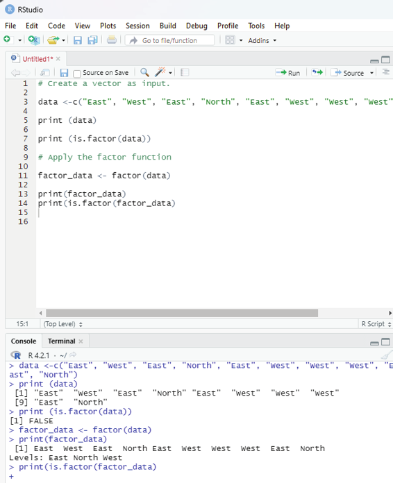

# Create a vector as input.
data <-c(“East”, “West”, “East”, “North”, “East”, “West”, “West”, “West”, “East”, “North”) print (data)
print (is.factor(data))
# Apply the factor function
factor_data <- factor(data)
print(factor_data)
print(is.factor(factor_data)
Image showing use of R factor
Prof. Dr Balasubramanian Thiagarajan
109
There are two steps involved in creating a factor: 1. Creating a vector
2. converting the created vector into a factor using the function factor() The user desires to create a factor gender with two levels i.e., male and female.
# Creating a vector
x<-c(“Female”, “Male”, “Male”, “Female”)
print (x)
# Converting the vector x into a factor.
# named gender
gender <-factor(x)
print(gender)
Output:
> x<-c(“Female”, “Male”, “Male”, “Female”)
> print (x)
[1] “Female” “Male” “Male” “Female”
> gender <-factor(x)
> print(gender)
[1] Female Male Male Female
Levels: Female Male
One can use the function levels() to check the level of the factor.
Accessing elements of a Factor in R:
It is something like accessing elements of a vector. The same principle is used to access the elements of a factor.
gender <- factor (c( “female”, “male”, “male”, “female”, “female”)); gender [3]
Output:
[1] male
Levels: female male
R Programming in Statistics


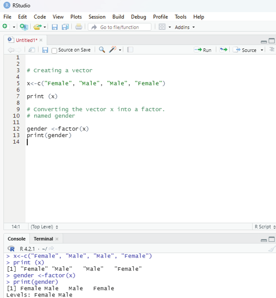

Image showing another example of the use of R factor
Prof. Dr Balasubramanian Thiagarajan
111


More than one element can also be accessed at a time.
gender[c(2,4)]
Output:
[1] male female
Levels: female male
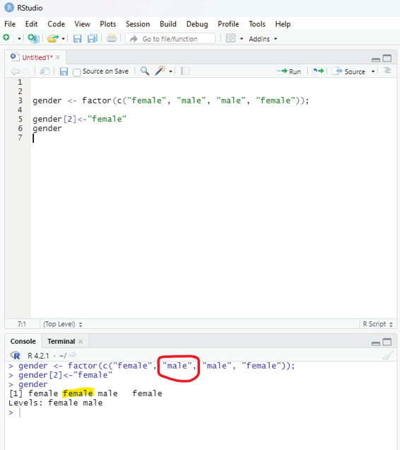
Modification of a factor in R:
After forming a factor, its components can be modified. The new values that needs to be assigned must be at the predefined level. If the value is gender then the new value should also be gender.
gender <- factor(c(“female”, “male”, “male”, “female”)); gender[2]<-”female”
gender
Image showing modification of a factor in R
R Programming in Statistics


Output:
[1] female female male female
Levels: female male
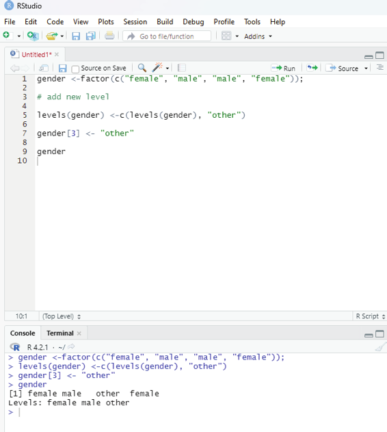
The user can also add a new level to the factor.
In this example a new level “other” needs to be added to the gender.
gender <-factor(c(“female”, “male”, “male”, “female”));
# add new level
levels(gender) <-c(levels(gender), “other”)
gender[3] <- “other”
gender
Image showing adding a new level to a factor
Prof. Dr Balasubramanian Thiagarajan
113
[1] female male other female
Levels: female male other
Lists:
These are the R objects that contain elements of different data types like - number, strings, vectors and another list inside it.
Syntax - list(data)
Example: Running this code in the script window will provide the list of the elements inside the three vectors in the list.
vtr1 <-c(1:5)
vtr2 <-c(“hi”, “hel o”, “How are you”)
vtr3 <-c(TRUE,TRUE,FALSE,FALSE)
myList <-(vtr1,vtr2,vtr3)
Using List function all data retain their original data type. They dont get converted into common data format. If the user wants to use multiple data types without resorting to conversion to a common data type then list function should be used.
R Programming in Statistics
Example: Running this code in the script window will provide the list of the elements inside the three vectors in the list.
vtr1 = c(1:5)
vtr2 = c(“hi”, “hel o”, “How are you”)
vtr3 = c(TRUE,TRUE,FALSE,FALSE)
myList <-c(vtr1,vtr2,vtr3)
Using List function all data retain their original data type. They dont get converted into common data format. If the user wants to use multiple data types without resorting to conversion to a common data type then list function should be used.
Note:
Various assignment operators are used in this example. They include =c and <-c. This is just to indicate both these operators can be used interchangeably. Operators will be discussed in detail in ensuing chapters.
Output:
myList
[1] “1” “2” “3” “4”
[5] “5” “hi” “hello” “How are you”
[9] “TRUE” “TRUE” “FALSE” “FALSE”
Using List function all data retain their original data type. They dont get converted into common data format. If the user wants to use multiple data types without resorting to conversion to a common data type then list function should be used.
A list can also contain a matrix or a function as its elements. List is created using list() function.
Example:
# Create a list containing strings, numbers, vectors and # a logical value.
list_data <- list(“Red”, “Green”,”Blue”, c(21,32,11), TRUE, 51.23, 119.1) print(list_data)
Prof. Dr Balasubramanian Thiagarajan
115


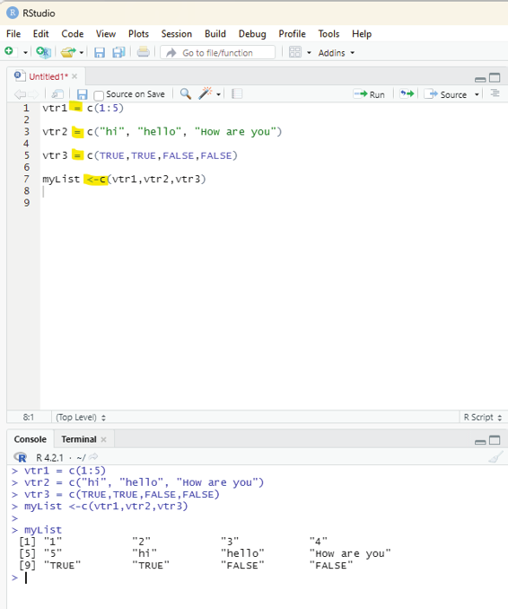

Image showing a list being formed with vectors containing numerical values, character values and Logical values.
R Programming in Statistics
[[1]]
[1] “Red”
[[2]]
[1] “Green”
[[3]]
[1] “Blue”
[[4]]
[1] 21 32 11
[[5]]
[1] TRUE
[[6]]
[1] 51.23
[[7]]
[1] 119.1
Output:
$`1st Quarter`
[1] “March” “April” “June”
$A_Matrix
[,1] [,2] [,3]
[1,] 4 3 10
[2,] 6 -1 7
$À Inner list`
$À Inner list`[[1]]
[1] “Yellow”
$À Inner list`[[2]]
[1] 11.2
Naming List elements:
The list elements can be given names and they can be accessed using these names.
Prof. Dr Balasubramanian Thiagarajan
117
Image showing a list containing a vector and a matrix
R Programming in Statistics


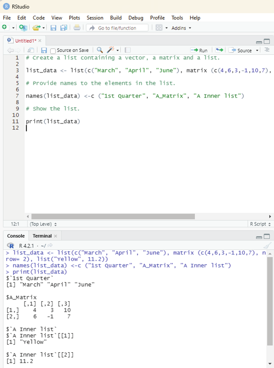

Image showing list elements being named
Prof. Dr Balasubramanian Thiagarajan
119
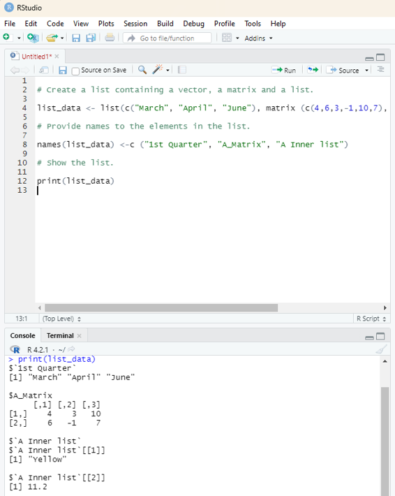
# Create a list containing a vector, a matrix and a list.
list_data <- list(c(“March”, “April”, “June”), matrix (c(4,6,3,-1,10,7), nrow= 2), list(“Yel ow”, 11.2))
# Provide names to the elements in the list.
names(list_data) <-c (“1st Quarter”, “A_Matrix”, “A Inner list”)
# Show the list.
print(list_data)
Output generated is shown below:
$`1st Quarter`
[1] “March” “April” “June”
$A_Matrix
[,1] [,2] [,3]
[1,] 4 3 10
[2,] 6 -1 7
$À Inner list`
$À Inner list`[[1]]
[1] “Yellow”
$À Inner list`[[2]]
[1] 11.2
Accessing list elements:
Elements can be accessed by the index of the element in the list. In case the lists are named then it can also be accessed using the names.
R Programming in Statistics


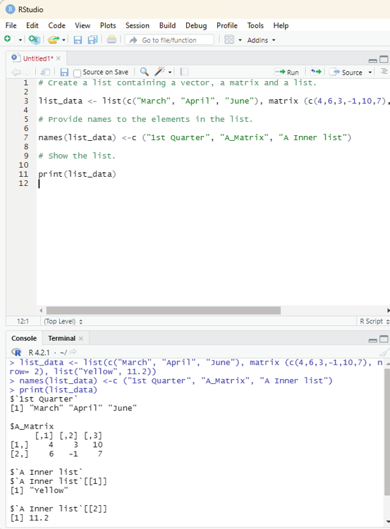

Image showing list elements being accessed
Prof. Dr Balasubramanian Thiagarajan
121
# Create a list containing a vector, a matrix and a list.
list_data <- list(c(“March”, “April”, “June”), matrix (c(4,6,3,-1,10,7), nrow= 2), list(“Yel ow”, 11.2))
# Provide names to the elements in the list.
names(list_data) <-c (“1st Quarter”, “A_Matrix”, “A Inner list”)
# Show the list.
print(list_data)
Output:
$`1st Quarter`
[1] “March” “April” “June”
$A_Matrix
[,1] [,2] [,3]
[1,] 4 3 10
[2,] 6 -1 7
$À Inner list`
$À Inner list`[[1]]
[1] “Yellow”
$À Inner list`[[2]]
[1] 11.2
# Give names to the elements in the list.
names(list_data) <- c(“1st Quarter”, “A_Matrix”, “A Inner list”)
# Access the first element of the list.
print(list_data[1])
# Access the thrid element. As it is also a list, all its elements will be printed.
print(list_data[3])
R Programming in Statistics
# Access the list element using the name of the element.
print(list_data$A_Matrix)
When the code is executed the following will be the result displayed: $`1st Quarter`
[1] “March” “April” “June”
> print(list_data$A_Matrix)
[,1] [,2] [,3]
[1,] 4 3 10
[2,] 6 -1 7
The list elements can also be manipulated:
One can add delete and update list elements. One can add and delete elements only at the end of a list. But one can update any element.
# Create a list containing a vector, a matrix and a list.
list_data <-list(c(“Jan”, “Feb”, “Mar”), matrix (c(2,4,6,2,-5,8), nrow=2),list(“blue”, 10.2))
# Give names to the elements in the list.
names(list_data) <-c(“1st Quarter”, “A_Matrix”, “A Inner list”)
# Add element at the end of the list.
list_data[4] <- “New element”
print(list_data[4])
# Update the 3rd element
list_data[3] <- “updated element”
print(list_data[3])
Merging lists:
Lists can be merged into one list by placing all the lists inside one list() function.
Prof. Dr Balasubramanian Thiagarajan
123


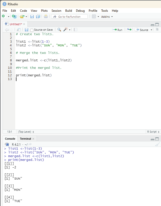

Image showing how to merge two lists
R Programming in Statistics
list1 <-list(1-3)
list2 <-list(“SUN”, “MON”, “TUE”)
# Merge the two lists.
merged.list <-c(list1,list2)
#Print the merged list.
print(merged.list)
On running the code the following output will be generated:
[[1]]
[1] 1
[[2]]
[1] 2
[[3]]
[1] 3
[[4]]
[1] “SUN”
[[5]]
[1] “MON”
[[6]]
[1] “TUE”
Converting list to vector:
A list can be converted to a vector so the events of the vector can be used for further manipulation. All the arithmetic operations on vectors can be applied after the list is converted into vectors. In order to make use of this feature one should use the unlist() function. It takes the list as the input and produces a vector.
Prof. Dr Balasubramanian Thiagarajan
125


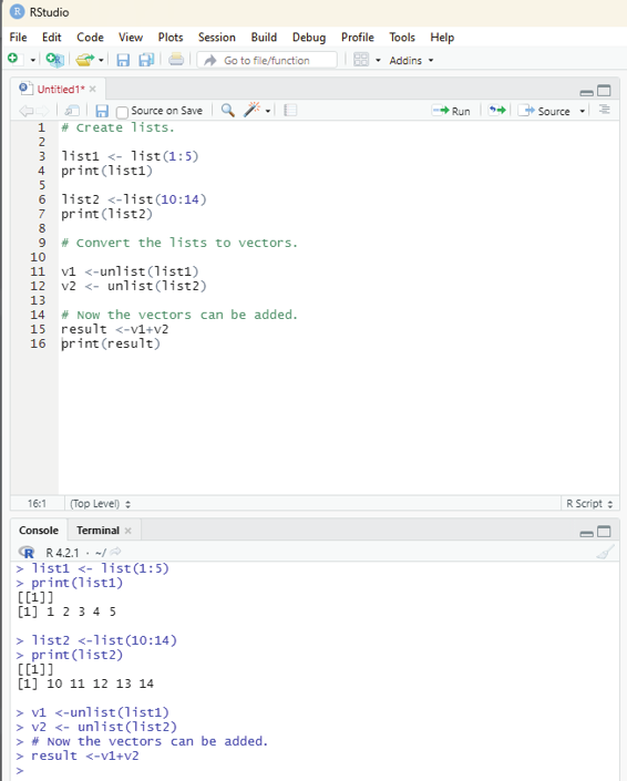

Image showing list converted to vector
R Programming in Statistics
list1 <- list(1:5)
print(list1)
list2 <-list(10:14)
print(list2)
# Convert the lists to vectors.
v1 <-unlist(list1)
v2 <- unlist(list2)
# Now the vectors can be added.
result <-v1+v2
print(result)
On running the code the following result will be displayed:
[1] 11 13 15 17 19
Data frame:
Data frames are data displayed in a format as a table.
Data frames can have different types of data inside it. While the first column can be “character”, the second and third can be “numeric” or “logical”. However, each column should have the same type of data.
This is a table or a two-dimensional array like structure in which each column contains values of one variable and each row contains one set of values from each column.
syntax - data.frame(data)
The following are the characteristics of a data frame:
1. The column names should not be empty
2. The row names should be unique
3. The data stored in a data frame can be of numeric, factor or character type 4. Each column should contain the same number of data items Example:
The aim is to create a data frame with the following data:
Prof. Dr Balasubramanian Thiagarajan
127
Pulse rate
Duration
Code:
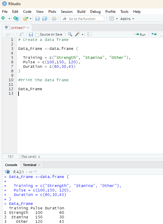
# Create a data frame
Data_Frame <-data.frame (
Training = c(“Strength”, “Stamina”, “Other”),
Pulse = c(100,150, 120),
Duration = c(60,30,45)
)
#Print the data frame
Data_Frame
Output:
Training Pulse Duration
1 Strength 100 60
2 Stamina 150 30
3 Other 120 45
In order to get summary of the data the following code can be used: output <-summary(Data_Frame)
> print(output)
Output:
Training Pulse Duration
Length:3 Min. :100.0 Min. :30.0
Class :character 1st Qu.:110.0 1st Qu.:37.5
Mode :character Median :120.0 Median :45.0
Mean :123.3 Mean :45.0
3rd Qu.:135.0 3rd Qu.:52.5
Max. :150.0 Max. :60.0
R Programming in Statistics
Image showing data frame being created using RStudio
Prof. Dr Balasubramanian Thiagarajan
129
Items from data frame can be accessed suing [] single brackets, [[]] double brackets, or $ symbol.
Example:
Data_Frame<- data.frame(
Training = c(“strength”, “stamina”, “other”),
Pulsee = c(100, 150, 120),
Duration = c(60,30,45)
)
Data_Frame [1]
Data_Frame[[“Training”]]
Data_Frame$Training
Code:
# Create the data frame.
emp.data <-data.frame(
emp_id = c (1:5),
emp_name = c(“John”, “Murphy”, “Sundar”, “Ramesh”, “Bony”), salary = c(600, 528.49, 789,854.8, 658),
start_date = as.Date (c(“2012-05-06”, “2012-06-22”, “2013-03-22”, “2015-04-16”,”2016-02-1”)),
stringsAsFactors = FALSE
)
# Print/display data frame
print(emp.data)
Structure of the data frame can be seen by using str() function.
str(emp.data)
R Programming in Statistics
Summary of Data in Data Frame:
The statistical summary and nature of the data can be obtained by applying summary() function.
Data can be extracted from Data Frame by using column name.
#Extract Specific Columns.
result <-data.frame(emp.data$emp_name, emp.data$salary) The user can also extract the first two rows and then all columns.
Code:
#Extract first two rows.
result <- emp.data[1:2,]
print (result)
print(result)
# Extract 3rd and 5th row with 2nd and 4th column.
result <- emp.data[c(3,5),c(2,4)]
print(result)
One can Expand Data Frame by adding columns and rows. code for adding column:
#Add the”dept” column
emp.data$dept <- c(“IT”,”Operations”, “IT”, “HR”, “Finance”) v <-emp.data
print (v)
Adding rows to the existing data frame:
To add more rows permanently to an existing data frame, one needs to bring in new rows in the same structure as the existing data frame. For this purpose rbind() function can be used.
Adding Rows using rbind() function:
Example:
Data_Frame <-data.frame(
Training = c(“Strength”, “Stamina”, “Other”),
Pulse = c(100,150,120),
Duration = c(60,30,45))
Prof. Dr Balasubramanian Thiagarajan
131
New_row_DF <- rbind(Data_Frame, c(“Strength”, 110, 110))
# Print the new row
New_row_DF
Add columns:
Extra columns can be added using cbind() function in a data frame.
Example:
Data_Frame <- data.frame(
Training = c(“Strength”, “Stamina”, “other”),
Pulse = c(100, 150, 120),
Duration = c(60,35,40)
)
#Add a new column:
New_col_DF <- cbind (Data_Frame, Steps = c(1000,6000,2000))
# Print the new column.
New_col_DF
Output:
Training Pulse Duration Steps
1 Strength 100 60 1000
2 Stamina 150 35 6000
3 other 120 40 2000
# Create the second data frame
emp.newdata <-
data.frame(
emp_id = c (6:8),
emp_name = c(“Kumar”,”kurnal”,”Abhay”),
salary = c(578.0,722.5,632.8),
start_date = as.Date(c(“2013-05-21”,”2013-07-30”,”2014-06-17”)), dept = c(“IT”,”Operations”,”Fianance”),
stringsAsFactors = FALSE
)
R Programming in Statistics
emp.finaldata <- rbind(emp.data,emp.newdata)
print(emp.finaldata)
Removing rows and columns in a Data Frame:
In order to remoe rows and columns c() function can be used.
Example:
Data_Frame <- data.frame (
Training =c(“Strength”, “Stamina”, “Other”),
Pulse =c(100,130,120),
Duration = c(60,30,20)
)
# Remove the first row and column.
Data_frame_new <- Data_Frame[-c(1), -c(1)]
# Print the new data frame
Data_frame_new
Output:
Pulse Duration
2 130 30
3 120 20
Amount of Rows and Columns in Data frame:
Amount of rows and columns in a Data frame can be ascertained using dim() function.
Example:
Data_Frame <-data.frame (
Training = c(“Strength”, “Stamina”, “Other”),
Pulse = c(100,120,110),
Duration = c(25, 40, 60)
)
dim(Data_Frame)
Prof. Dr Balasubramanian Thiagarajan
133


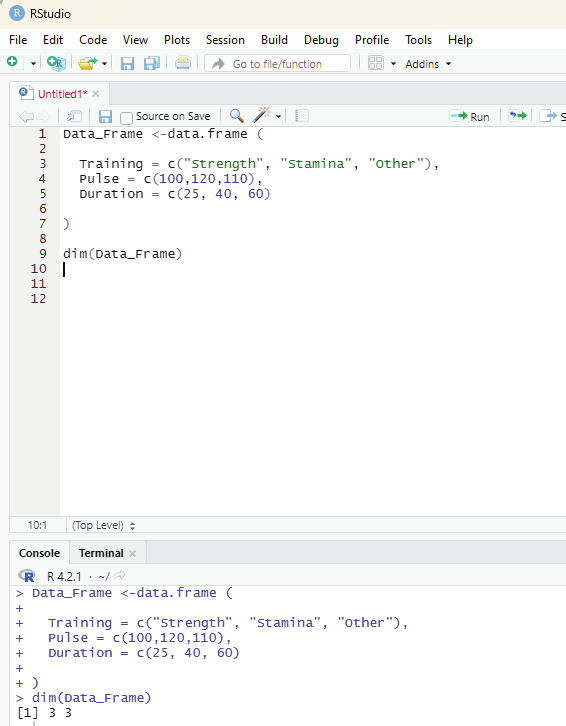

Output:
[1] 3 3
Image showing estimating the number of rows and columns using RStudio R Programming in Statistics
One can also use the ncol() function to find the number of columns and nrow() function to find the number of rows.
ncol(Data_Frame)
nrow(Data_Frame)
Output:
> ncol(Data_Frame)
[1] 3
>
> nrow(Data_Frame)
[1] 3
Data Frame Length:
In order to ascertain the number of columns in a Data frame length() function can be used (similar to ncol() function).
length(Data_Frame)
Output:
length(Data_Frame)
[1] 3
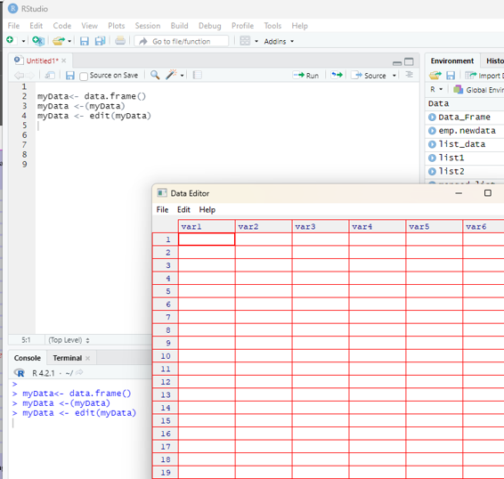
R does not have a spread sheet type of data entry facility. (Something similar to that of Excel). There are ways to invoke a speadsheet like data entry tool in R.
First step:
Object must be created. Everything in R is considered to be an object and this is actual y the fundamental distinction between R and Excel. While one can launch a spreadsheet like viewer for data entry in R, one needs to pass the data into an object. In order to do this a blank data frame needs to be setup with rows and columns. If the user leaves the arguments blank in data.frame it would result in an empty data frame.
myData<- data.frame()
Second step:
Data is edited in the viewer.
One has to use the edit function to launch the viewer. The user should pass the myData data frame bak to the myData object. In this way the changes made to the module will be saved to the original object.
Prof. Dr Balasubramanian Thiagarajan
135
myData <-(myData)
myData <- edit(myData)
The variable names can be changed by clicking on their labels and typing the changes. One can also set variables as numeric or character.
Note - One cannot set a variable to logical; and it has to be done in the syntax editor.
On data being entered, they get saved automatical y.
Third step:
Image showing Data Editor window opening
R Programming in Statistics


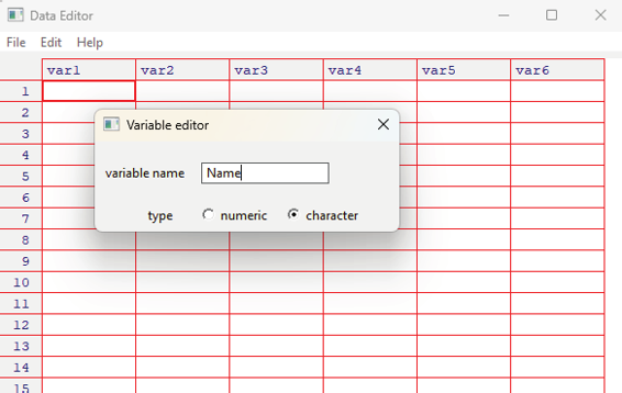

Data Entry in the spreadsheet format:
In order to change the header name the user needs to click on it. Input window will open prompting the user to key in a new name for the chosen column. The type of data that needs to be entered can also be chosen from this input window. The user has the option of choosing between character and Numerical formats.
Image showing the variable editor input window that appears on clicking the header of the column. In this image in the variable name column the desired value is entered. In the type of data the desired type of data is also choosen (numeric and character).
Variable editor does not provide the option of naming the data type as logical. This needs to be done at the level of syntax editor using the following command:
myData
is.logical(myData$IsInjured)
myData$IsInjured <- as.logical(myData$IsInjured)
This syntax is specifical y for the example given. The user can change the name of the data in the syntax before executing. This example is provided with an intention that the user should familiarize themselves with various syntax that can be used in R.
Prof. Dr Balasubramanian Thiagarajan
137


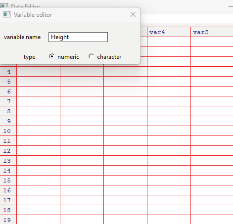


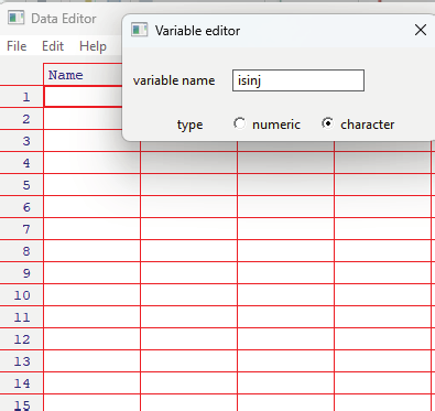

Image showing second variable name being changed to Height and the type of data that is to be entered in this column is chosen as numeric.
Image showing the third variable name changed to reflect the status whether injured or not. Type of data eventhough it is logical cannot be specified here. Only character needs to be choosen.
R Programming in Statistics


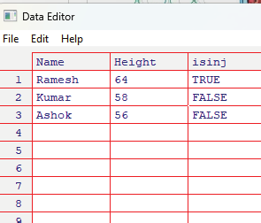

Data can be entered in each of these columns as shown below.
When the table is closed it automatical y gets saved.
As stated earlier the data editor does not set the columns to logical. It can be assigned only using the syntax editor.
Code for setting the columns as logical:
myData
is.logical(myData$IsInjured)
myData$IsInjured <- as.logical(myData$IsInjured)
Full code:
#create blank data frame
myData <- data.frame()
#edit data in the viewer
myData <- edit(myData)
#close & load
myData
#change IsInjured to Logical
is.logical(myData$IsInjured)
myData$IsInjured <- as.logical(myData$IsInjured)
Prof. Dr Balasubramanian Thiagarajan
139
Operators are symbols that tels the compiler to perform specific mathematical or logical computations. R
language is rich in built-in operators and provides the following types of operators: 1. Arithmetic operators
2. Relational operators
3. Logical operators
4. Assignment operators
5. Miscel aneous operators
Arithmetic operators:
These operators are used to perform arithmetic calculations. They include:
+ Adds two vectors
- Subtracts the second vector from the first
* Multiplies both vectors
/ Divide the first vector with the second
%% Divide the first vector with the second and display the remainder
%/% It provides the result of division of first vector with second one (quotient).
^ The first vector is raised to the exponent of second vector.
R Programming in Statistics


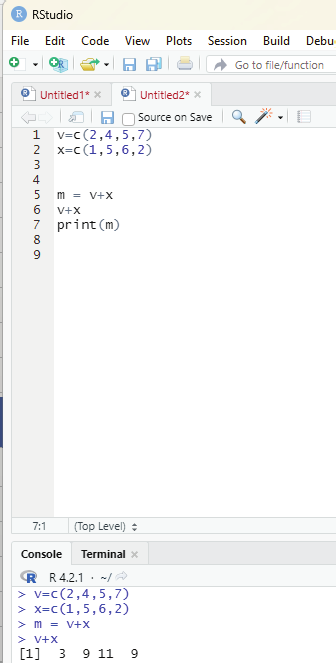

Addition:
In this example two vectors v and x are created holding a series of numbers. The intention is to add the numbers in the first vector (v) with that of the second (x) and display the result.
Code:
v=c(2,4,5,7)
x=c(1,5,6,2)
m = v+x
v+x
print(m)
Prof. Dr Balasubramanian Thiagarajan
141


Output:
[1] 3 9 11 9
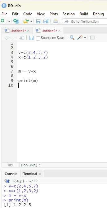
Subtraction:
In this example two vectors v and x are created holding a series of numbers. The intention is to subtract the numbers in the second vector x from the first vector v and display the result.
Code:
(c next to = sign is an assignment operator. It will be discussed later under assignment operators.
v=c(2,4,5,7)
x=c(1,2,3,2)
m = v-x
print(m)
Image showing the subtraction code executed in RStudio
R Programming in Statistics
Output:
[1] 1 2 2 5
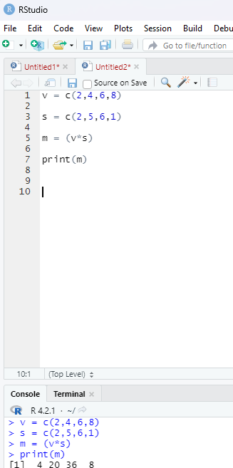
Multiplication operator:
* - Multiplies both vectors
Example:
v = c(2,4,6,8)
s = c(2,5,6,1)
m = (v*s)
print(m)
Output generated on running the code:
[1] 4 20 36 8
Image showing multiplication operator in use
Prof. Dr Balasubramanian Thiagarajan
143
Division operator:
/ - This operator divides the first vector with the second.
# Create two vectors with four numbers each.
x = c(2,5,4,34)
y = c(1,5,3,12)
z = (x/y)
print(z)
Output:
2.000000 1.000000 1.333333 2.833333
Dividing the first vector with the second vector and displaying only the remainder.
The operator used for this purpose is %%.
Example:
In this example two variables x and y are created. Numerical values are assigned to each of these variables.
The first variable x is divided with the second variable y. The remainder is displayed if %% operator is used.
Code:
x = 5
y = 2
print(x%%y)
Output:
[1] 1
R Programming in Statistics


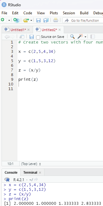

Image showing division operator being used
Prof. Dr Balasubramanian Thiagarajan
145


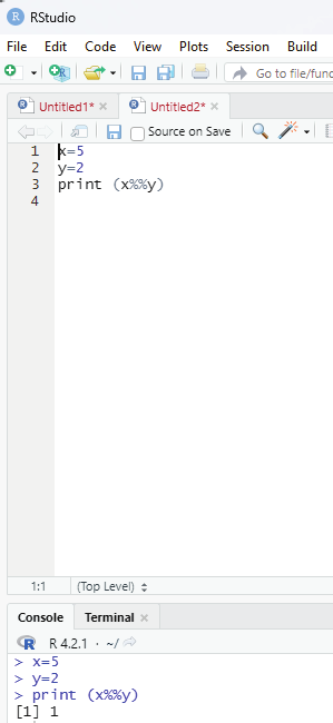

Image showing division operator with display of remainder
R Programming in Statistics
Example showing the role of %% in vectors containing a number of numeric variables.
Code:
x= c(5, 3, 4, 6)
y=c( 2, 2, 3, 2)
print (x%%y)
Output:
1 1 1 0
Code for the result of division of first vector with that of second. Displaying only the quotient and not the remainder.
x = c(3,6,8,7)
y = c(2,3,6,3)
m = (x%/%y)
print(m)
Output: 1 2 1 2
Prof. Dr Balasubramanian Thiagarajan
147


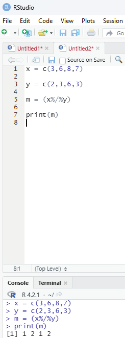

Image showing quotient being displayed after performing the division. The operator used is %/%
R Programming in Statistics
Exponent is defined as the number of times a number is multiplied by itself.
Example 2 to the third exponent means 2x2x2 = 8.
Code:
x = c(2,5,5,6)
y = c(2,3,4,2)
z = (x^y)
print(z)
Output:
4 125 625 36
Relational operators:
In this each element of the first vector is compared with that of the corresponding element of the second vector. the result of this comparison is a Boolean value. Given below are the list of various relational operators.
> Checks if each element of the first vector is greater than the corresponding element of the second vector.
< Checks if each element of the first vector is less than the corresponding element of second vector.
== Checks if each element of the first vector is equal to the corresponding element of the second vector.
<= Checks if each element of the first vector is less than or equal to the corresponding element of the second vector.
>= Checks if each element of the first vector is greater than or equal to the corresponding element of the second vector.
!= Checks if each element of the first vector is unequal to the corresponding element of second vector.
Prof. Dr Balasubramanian Thiagarajan
149


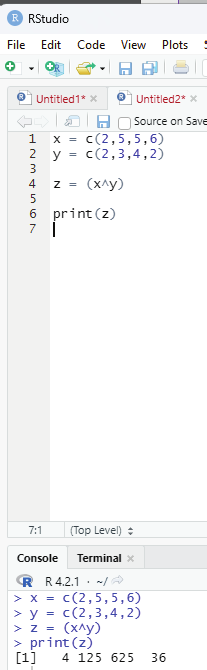

Image showing the use of exponent operator in R programming R Programming in Statistics
Logical operators: These are symbol / word used to connect two or more expressions such that the value of the compound expression produced depends only on that of the original expressions and on the meaning of the operator. Common logical operators include AND, OR and NOT.
& - It is known as Element-wise Logical AND operator. It combines each element of the first vector with that of the corresponding element of the second vector and gives a output TRUE if both the elements are TRUE.
| - It is cal ed Element-wise Logical OR operator. It combines each element of the first vector with the corresponding element of the second vector and gives a output TRUE if one of the elements is TRUE.
! - It is known as Logical NOT operator. It takes each element of the vector and gives the opposite logical value.
&& - It is cal ed logical AND operator. It takes the first element of both the vectors and gives the TRUE only if both are TRUE.
|| - It is caLLED Logical OR operator. It takes the first element of both the vectors and gives the TRUE if one of them is TRUE.
Example for > (greater than):
Code:
x = c(4,6,8,9)
y = c(3,5,7,9)
print(x>y)
Output:
TRUE TRUE TRUE FALSE
Output reveals that first element of first vector of greater than the first element of second vector - hence the value TRUE.
The second element of first vector is greater than the second element of second vector - hence the value TRUE
The third element of first vector is greater than the third element of second vector - hence the value TRUE.
The fourth element of first vector is less than the fourth element of second vector - hence the value FALSE.
Prof. Dr Balasubramanian Thiagarajan
151


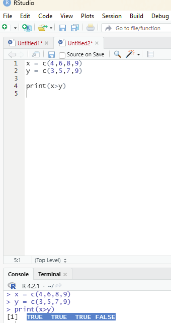

Image showing the use of > (greater than operator)
R Programming in Statistics
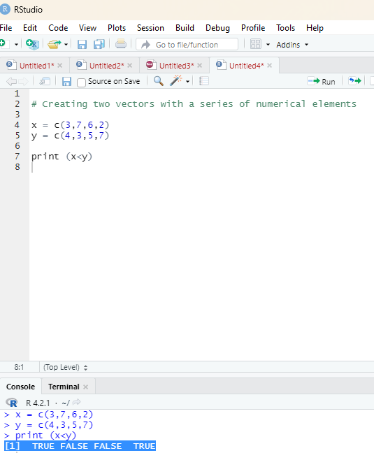
Example for < (lesser than):
Code:
Code:
x = c(3,7,6,2)
y = c(4,3,5,7)
print (x<y)
Output:
[1] TRUE FALSE FALSE TRUE
Prof. Dr Balasubramanian Thiagarajan
153
Study of output reveals :
The first element of vector x is less than that of the first element of vector y. Hence the value TRUE is printed.
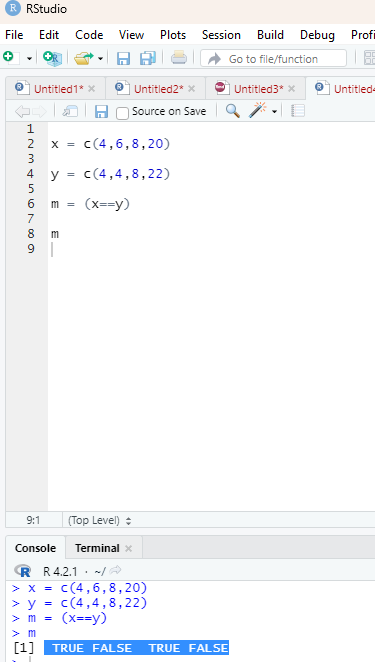
Check to find if each element of the first vector is equal to the corresponding element of the second vector: Operator - ==
Code:
x = c(4,6,8,20)
y = c(4,4,8,22)
m = (x==y)
m
Output: TRUE FALSE TRUE FALSE
Image showing the use of == operator
R Programming in Statistics
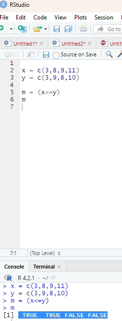
Operator that is used to check if each element of the first vector is less than or equal to the corresponding element of the second vector:
Operator used:
<=
Code:
x = c(3,8,9,11)
y = c(3,9,8,10)
m = (x<=y)
Output : TRUE TRUE FALSE FALSE
Image showing the use of <= operator
Prof. Dr Balasubramanian Thiagarajan
155


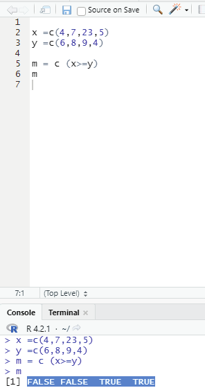

Operator to check if each element of the first vector is greater than or equal to the corresponding element of the second vector.
Operator used:
>=
Code:
x =c(4,7,23,5)
y =c(6,8,9,4)
m = c (x>=y)
Output : FALSE FALSE TRUE TRUE
Image showing the use of >= operator
R Programming in Statistics


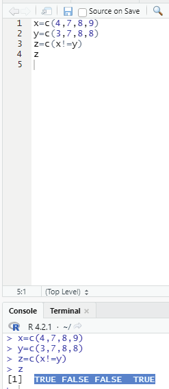

Operator to check if each element of the first vector is unequal to the corresponding element of the second vector.
Operator:
!=
Code:
x=c(4,7,8,9)
y=c(3,7,8,8)
z=c(x!=y)
z
Output:
TRUE FALSE FALSE TRUE
Image showing the use of !=
Prof. Dr Balasubramanian Thiagarajan
157
Given below are the various logical operators supported in R language. It is applicable only to vectors of type logical, numeric or complex. All numbers greater than 1 is considered as logical value true.
Operator: &
This operator is called Element wise logical AND operator. It combines each element of the first vector with the corresponding element of the second vector and gives an output TRUE if both the elements are TRUE.
Code:
x = c(2,4,0, TRUE, 2+3i)
y = c(3,0,1, FALSE, 2+3i)
z = c(x&y)
z
Output:
TRUE FALSE FALSE FALSE TRUE
Considering the output the following explanation can be offered: When the first value of both vectors are compared it can be seen both these values are more than 1 and hence both values are supposed to be TRUE. Since both values are TRUE the output generated shows the value TRUE.
When the second value of both vectors are compared it can be seen that the first vector has a value of more than one (hence should show TRUE, while the second value of the second vector is less than 1 and hence should display the value FALSE. Since both these values are not similar the output displays the value FALSE
Similary the third value of both vectors displays disimilar logical values hence they are reported in the output as FALSE.
The last value of the First and Second vectors are both more than 1 and hence the output displays the value TRUE.
R Programming in Statistics


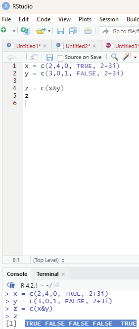

Image showing the use of & operator
Prof. Dr Balasubramanian Thiagarajan
159


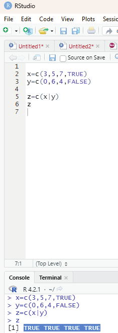

Operator: |
This is also known as element wise logical OR operator. It combines each element of the first vector with the corresponding element of second vector and gives an output as TRUE if one of the elements is TRUE.
Code:
x=c(3,5,7,TRUE)
y=c(0,6,4,FALSE)
z=c(x|y)
z
Output:
TRUE TRUE TRUE TRUE
Image showing the use of or operator
R Programming in Statistics


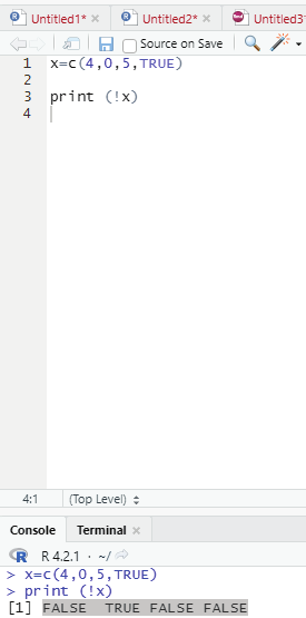

Operator: !
This operator is also known as logical NOT operator. This operator takes each element of the vector and gives the opposite logical value.
Code:
x=c(4,0,5,TRUE)
print (!x)
Output:
FALSE TRUE FALSE FALSE
Image showing the use of NOT operator
Prof. Dr Balasubramanian Thiagarajan
161
The logical operators && and || considers only the first element of the vectors and give a vector of single element as output.
Operator - &&
This operator is also known as Logical AND operator. It takes the first element of both the vectors and gives the TRUE only if both are true.
Code:
v <- c(3,0,TRUE,2+2i)
t <- c(1,3,TRUE,2+3i)
print(v&&t)
Output:
TRUE
Operator ||:
This is also known as Logical OR operator. This operator takes the first element of both the vectors and gives the TRUE if one of them is TRUE.
Code:
v <- c(0,0,TRUE,2+2i)
t <- c(0,3,TRUE,2+3i)
print(v||t)
Output:
FALSE
Some of the other mathematical functions are:
Square root - sqrt
Logarithm - log
Exponential - exp
R Programming in Statistics


Reader is encouraged to try out all these functions.
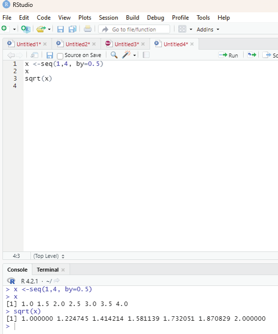
# Create a vector “x” with a sequence of numbers between 1 and 4. These numbers should increment by 0.5.
Code:
x <-seq(1,4, by=0.5)
x
sqrt(x)
Output:
x <-seq(1,4, by=0.5)
> x
[1] 1.0 1.5 2.0 2.5 3.0 3.5 4.0
> sqrt(x)
[1] 1.000000 1.224745 1.414214 1.581139 1.732051 1.870829 2.000000
>
Image showing the above code in execution
Prof. Dr Balasubramanian Thiagarajan
163
Similary Logarithmic value of x can be calculated using log command.
log(x)
Sine value can be calculated using sin command.
sin(x)
Output:
> log(x)
[1] 0.0000000 0.4054651 0.6931472 0.9162907 1.0986123 1.2527630 1.3862944
> sin(x)
[1] 0.8414710 0.9974950 0.9092974 0.5984721 0.1411200 -0.3507832
[7] -0.7568025
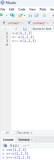
Assignment Operators:
These operators are used to assign values to vectors.
Left assignment:
<-
=<<-
These operators can be used interchangeably.
v=c(1,2,3)
v<-c(1,2,3)
v<<-c(1,2,3)
c indicates concatenate in R language.
R Programming in Statistics
Image showing left assignment operators in use. They can be used interchangeably.
Prof. Dr Balasubramanian Thiagarajan
165
Right assignment operators:
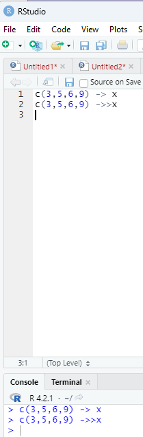
->
Example:
c(3,5,6,9) -> x
Note the code is reversed.
->>
c(3,5,6,9) ->>x
R Programming in Statistics


Miscel aneous operators:
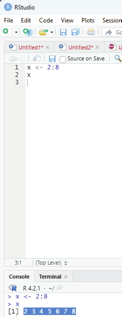
: (colon operator): This operator creates the series of numbers in sequence for a vector.
x <- 2:8
print (x)
Output:
2 3 4 5 6 7 8
Image showing colon operator
Prof. Dr Balasubramanian Thiagarajan
167
This operator is used to identify if an element belongs to a vector.
Example:
# Two vector are created.
x <-8
y <- 12
# Condition vector. Inside this vector the condition is entered, which is a series of numbers between 1 and 10
with an incremental value of 1 between them.
z <-1:10
print (x%in%z)
# This is to query whether variable x contains any value between 1 and 10.
print (y%in%z)
Output:
x <-8
> y <- 12
> z <-1:10
> print (x%in%z)
[1] TRUE
> print <-(y%in%z)
>
> print (y%in%z)
[1] FALSE
>
%*% Matrix multiplication:
This operator is used to multiply a matrix with its transpose.
Code:
M = matrix( c(2,6,5,1,10,4), nrow = 2,ncol = 3,byrow = TRUE) t = M %*% t(M)
print(t)
Output:
[,1] [,2]
[1,] 65 82
[2,] 82 117
R Programming in Statistics
There are many inbuilt functions in R that helps the researcher in data analysis. These are rather simple to use.
Function
Purpose
Mean
Mean
Median
Median
sd
Standard deviation
var
variance
mad
Median Absolute deviation
min
Minimum
max
maximum
Range
Range of values (minimum and maximum)
sum
Total sum
The first argument to all these functions is the data and should be single vector of values.
Example:
age<-c(24,34,12,56,72,84)
median(age)
Output : 45
mad(age)
Output : 35.5824
range (age)
Output: 12 84
If missing data is there in the vector values then extra care needs to be taken while running these functions.
When there are missing values in the vector values running these functions will give a return value of NA.
This can be avoided by using the argument na.rm = (TRUE/FALSE).
Example:
age<-c(24,34,12,56,72,NA)
median (age, na.rm=TRUE)
Output - 34
Prof. Dr Balasubramanian Thiagarajan
169


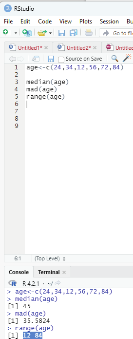


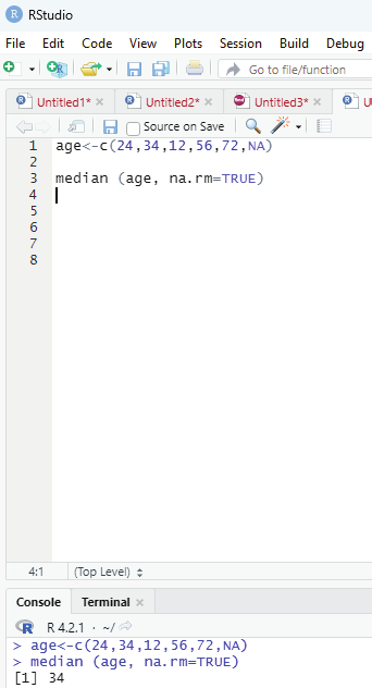

Image showing the use of various statistical summary functions Image showing how to handle missing data
R Programming in Statistics
Simulation and statistical distributions:
User who is working with statistical distributions in R, there are functions available for all of the common distributions and all common actions. All of these functions follow the same pattern of naming, which starts with a single letter to identify what the user wants to do and is followed by the R code name for the distribution.
R Code fot Statistical Distribution
Distribution
R Code
Distribution
R Code
Normal
norm
Poisson
pois
Binominal
binom
Exponential
exp
Uniform
unif
Weibull
weibull
Beta
beta
Gamma
gamma
F
f
Chi-squared
chisq
The list shown above is not a complete one. More can be found in the help pages by seaching for the name of the distribution. The user will have to combine the name of the distribution with a letter that determines whether to sample or calculate the quartiles.
Letter
Purpose
First Argument
Example
d
Probability density func-
x (qauntiles)
dnorm (1.64)
tion
p
Cumulative probability
q (quantiles)
pnorm (1.64)
density function
q
Quantile function
p (probabilities)
qnorm (0.95)
r
Random sampling
n (sample size)
rnorm (100)
Table showing various Distribution functions
Normal distribution has the arguments mean and sd that are set to the Standard Normal defaults (0 1nd 1) whereas the Poisson distribution has the argument lambda., which does not have a default value set. In general the arguments will be set to the “standard” values for the distribution. If the distribution does not have a standard, default values will not be set.
Example:
rnorm (5)
Output:
[1] 0.3321504 -0.1533315 -0.8361300 0.5362145 -1.6682728
Prof. Dr Balasubramanian Thiagarajan
171


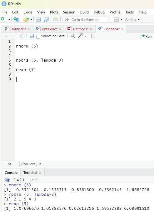

rpois (5, lambda=3)
Output:
[1] 2 1 5 4 3
rexp (5)
Output:
[1] 1.07696670 1.01383576 0.02613216 1.59532388 0.08991510
Image showing codes for various types of distribution
R Programming in Statistics
The above codes allows the user to simulate values from a distribution. If the user needs to generat3e samples from the existing data then the function sample should be used. This function allows the user to specify the vector the sample is desired from, the number of samples needed by the user, whether the user wants to replace the values or not, and whether the user desires to change the probability of sampling particular value, which are equal by default.
# As an example the function “sample” is applied to the vector of ages.
age = c(5,7,19,22,35,76,45,34)
sample (age, size =5)
Output:
[1] 45 35 34 76 5
Replace argument if used allows values to be sampled again when it is set to TRUE. If it is set to FALSE a value cannot be sampled again after it has been sampled once.
sample(age, size = 5, replace = TRUE)
Output:
[1] 76 76 5 22 45
Recreating simulated values in R Programming:
If the user desires to recreate the random samples from the samples one will need to set the random seed.
This can be done using function set.seed. This takes an integer value to indicate the seed to u se. This function can be used to change the type of random number generator used.
Example for generating random numbers from normal distribution: Random numbers from a normal distribution can be generated using rnorm() function. The user will have to specify the number of samples to be generated. One can also specify the mean and standard deviation of the distribution. If these values are not provided the distribution defaults to 0 mean and 1 standard deviation.
# Code to generate 1 random number
rnorm(1)
Output:
0.8418733
# Code to generate 3 random numbers.
rnorm (3)
Prof. Dr Balasubramanian Thiagarajan
173


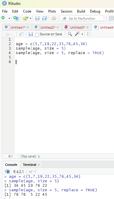

Image showing the use of sample function
R Programming in Statistics
0.6218214 -1.2239963 -1.5102920
Code to for providing the user’s own mean and standard deviation.
rnorm (3, mean=10, sd=2)
Output:
9.487026 8.168494 11.471801
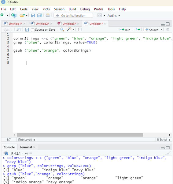
Search and Replace function:
These are two very useful functions for working with character data: grep - This function allows the user to search elements of a vector for a particular pattern.
gsub - This function replaces a particular pattern with a given string (gsub).
Example:
colorStrings <-c (“green”, “blue”, “orange”, “light green”, “indigo blue”, “navy blue”)
# Code to search for red in the above character string.
grep (“blue”, colorStrings, value=TRUE)
Output:
“blue” “indigo blue” “navy blue”
Search and Replace function:
These are two very useful functions for working with character data: grep - This function allows the user to search elements of a vector for a particular pattern.
gsub - This function replaces a particular pattern with a given string (gsub).
Example:
colorStrings <-c (“green”, “blue”, “orange”, “light green”, “indigo blue”, “navy blue”)
# Code to search for red in the above character string.
grep (“blue”, colorStrings, value=TRUE)
Prof. Dr Balasubramanian Thiagarajan
175
Output:
“blue” “indigo blue” “navy blue”
gsub (“blue”, ” orange”, colorStrings)
Output:
[1] “green” “orange” “orange” “light green”
[5] “indigo orange” “navy orange”
Image showing the use of grep and gsub functions
R Programming in Statistics
Functions in R allows the use to perform a number of tasks with a simple command. Writing functions is more or less similar with most programming languages. Creating own functions by the user is a powerful aspect of R. It allows the user to “wrap up” a series of steps into a simple container. In this way the user can capture common workflows and utilities and call them when needed instead of producing long, verbose scripts of repeated code snippets that can be difficult to manage. The function performs its task and returns control to the interpreter as well as any result which may be stored in other objects.
Components of Functions:
Function name - This is the name of the function. It is stored in R environment as an object with this name.
Arguments - An argument is a placeholder. When a function is invoked, a value is passed to the argument.
Arguments are optional; that is a function may contain no arguments. Arguments also can have default values.
Function Body - The function body contains a collection of statements that defines what the function does.
Return value - The return value of a function is the last expression in the funciton body to be evaluated.
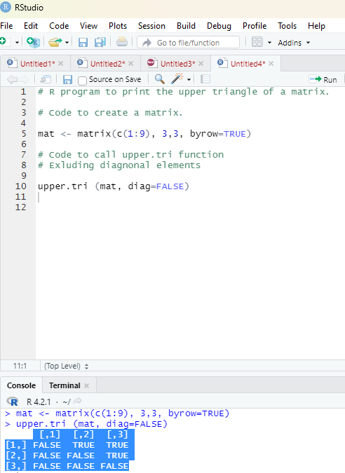
.upper.tri function:
This function allows the user to identify values in the upper triangle of a matrix.
Syntax: upper.tri(x,diag)
x: Matrix object
diag: Boolean value to include diagonal
Code:
# R program to print the upper triangle of a matrix.
# Code to create a matrix.
mat <- matrix(c(1:9), 3,3, byrow=TRUE)
# Code to call upper.tri function
# Exluding diagnonal elements
upper.tri (mat, diag=FALSE)
Prof. Dr Balasubramanian Thiagarajan
177
Output:
[,1] [,2] [,3]
[1,] FALSE TRUE TRUE
[2,] FALSE FALSE TRUE
[3,] FALSE FALSE FALSE
Image showing upper.tri function in use
R Programming in Statistics
Output showing the contents of the Matrix:
[,1] [,2] [,3]
[1,] 1 2 3
[2,] 4 5 6
[3,] 7 8 9
Output seen after using upper.tri (mat, diag=FALSE) code.
[,1] [,2] [,3]
[1,] FALSE TRUE TRUE
[2,] FALSE FALSE TRUE
[3,] FALSE FALSE FALSE
Output seen after using upper.tri(mat, diag = TRUE)
[,1] [,2] [,3]
[1,] TRUE TRUE TRUE
[2,] FALSE TRUE TRUE
[3,] FALSE FALSE TRUE
In mathematics (linear algebra), a triangular matrix is a special kind of square matrix. A square matrix is called lower triangular if all the entries above the main diagonal are zero. Similarly, a square matrix is called upper triangular if all the entries below the main diagonal are zero.
A square matrix is said to be lower trianglular matrix if all the elements above its main diagonal are zero.
A square matrix is said to be an upper triangular matrix if all the elements below the main diagonal are zero.
B = 2 0 0
1 5 0
1 1 2
(Lower triangular matrix)
A = 2 -1 3
0 5 2
0 0 2
(Upper triangular matrix)
Prof. Dr Balasubramanian Thiagarajan
179


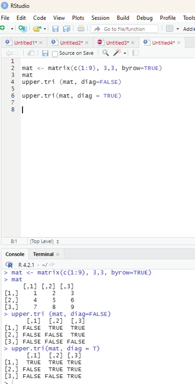

Image showing the use of upper.tri function with diag (true and false) arguments R Programming in Statistics
Functions typical y contains more than one line of code. The script window is preferred to the console window while developing functions.
Naming a function:
A function is an R object and hence can be named like any other R object. The name can be: Of any length.
Contain any combinations of letters, numbers, underscores and period characters.
Cannot start with a number.
Creating a simple function:
The user can create a simple function in R using the function keyword. Curly brackets are used to contain the body of the function.
Example:
addOne <- function (x) {x+1}
This function adds 1 to any input object.
addOne (x=2.5)
Output:
3.5
Types of functions in R language:
Built in function:
R has many in-built functions which can be directly called in the program without defining them first. One can also create and use customized functions referred to as user defined functions. Some of the in-built functions available in R are:
seq()
mean()
max()
sum(x)
paste(...)
Examples:
1. Creation of a sequence of numbers from 32 to 44.
print(seq(32,44))
Another command can be used to perform the same function using : Prof. Dr Balasubramanian Thiagarajan
181


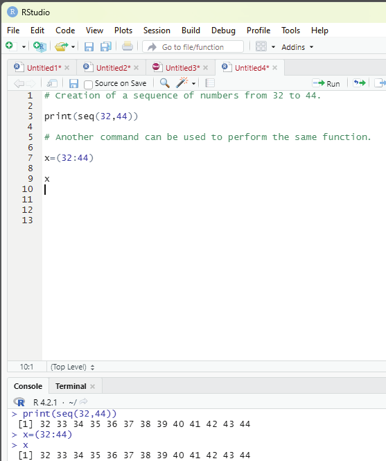

x = (32:44)
x
Image showing creation of sequence of numbers
R Programming in Statistics


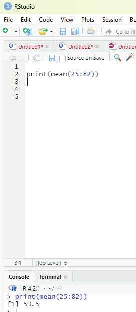

2. Finding mean of numbers from 25 to 82.
print(mean(25:82))
Output generated : 53.5
Image showing calculation of mean value of a series of numbers Prof. Dr Balasubramanian Thiagarajan
183
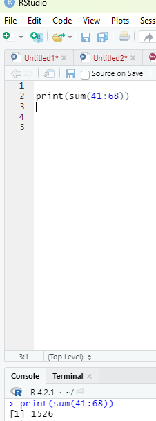
3. Finding sum of numbers from 41 to 68.
print(sum(41:68))
Output : 1526
Image showing the sum of a series of numbers calculated
R Programming in Statistics


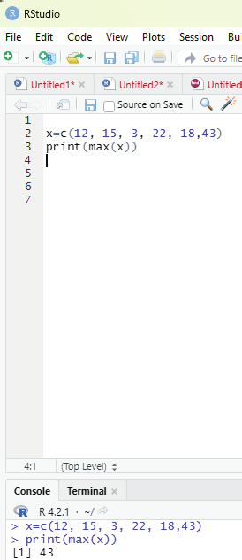

4. Finding the maximum from a series of values
x=c(12, 15, 3, 22, 18,43)
print(max(x))
4. Finding the maximum from a series of values
x=c(12, 15, 3, 22, 18,43)
print(max(x))
Output: 43
Image showing identifying the maximum value of a series of numbers Prof. Dr Balasubramanian Thiagarajan
185


Example of user defined function:
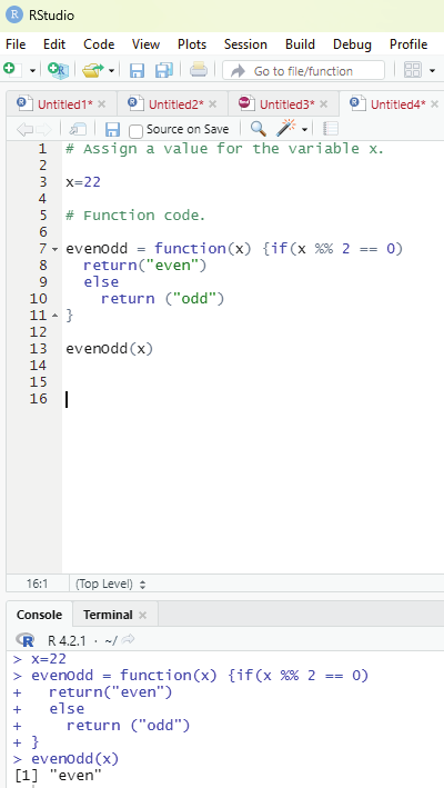
1. The aim of this function is to check whether the value assigned to the variable x is even or odd.
# Assign a value for the variable x.
x=22
# Function code.
evenOdd = function(x) {if (x %% 2 == 0)
return(“even”)
else
return (“odd”)
}
print (evenOdd(x))
Output: “even”
Image showing code that identifies odd and even numbers
R Programming in Statistics


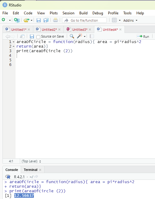

2. The aim is to create a function in R that will take a single input and gives a single output. This function code should calculate the area of a circle when the radius is fed. The name of the funcion that needs to be created is ‘areaOfCircle”, and the arguments that are needed to be passed are the “radius” of the circle.
Code:
areaOfCircle = function(radius){ area = pi*radius^2
return(area)}
print(areaOfCircle (2))
Outout: 12.56637
Image showing area of circle calculated
Prof. Dr Balasubramanian Thiagarajan
187


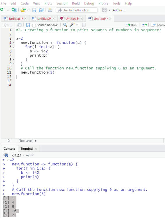

3. Creating a function to print squares of numbers in sequence: new.function <- function(a) {
for(i in 1:a) {
b <- i^2
print(b)
}
}
# Call the function new.function supplying 6 as an argument.
new.function(5)
Output:
[1] 1
[1] 4
[1] 9
[1] 16
[1] 25
Image showing the calculation of squares of numbers
R Programming in Statistics


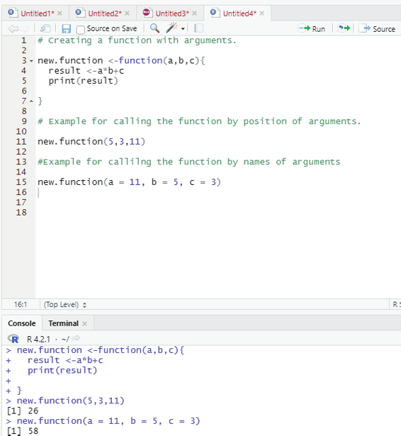

4. Calling a function with argument values (by position and by name).
The arguments to a function call can be supplied in the same sequence as defined in the funciton, or they can be supplied in a different sequence but assigned to the names of the arguments.
# Creating a function with arguments.
new.function <-function(a,b,c){
result <-a*b+c
print(result)
}# Example for calling the function by position of arguments.
new.function(5,3,11)
#Example for callilng the function by names of arguments
new.function(a = 11, b = 5, c = 3)
Image showing function with argument values by position and name Prof. Dr Balasubramanian Thiagarajan
189


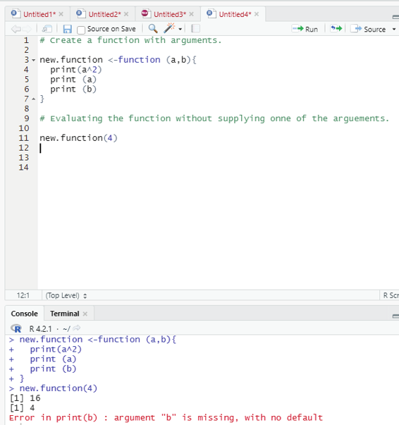

5. Lazy Evaluation of Function:
Arguments to functions are evaluated lazily. This means that they are evaluated only when needed by the function body.
# Create a function with arguments.
new.function <-function (a,b){
print(a^2)
print (a)
print (b)
}
# Evaluating the function without supplying onne of the arguements.
new.function(4)
This will actual y throw an error in printing b stating that argument “b” is missing.
Image showing laze evaluation function
R Programming in Statistics
Number of arguments in a function:
By default, a function must be called with the correct number of arguments. If the function expects 2 arguments, one will have to call the fucntion with two arguments, not more, and not less.
Example:
my_function <- function(fname, lname) {
paste(fname, lname)
}my_function(“Sam”, “Peter”)
Return values:
In order to make a function return a result the return() function should be used.
Example for the use of return() function:
multiplication_function <-function(x) {
return (5*x)
}
print (multiplication_function(2))
print (multiplication_function(4))
print (multiplication_function(5))
Nested functions:
There are two ways of creating Nested function.
1. Call a function within another function
2. Write a function within a function
Example - To call a function within another function:
Nested_function <- function(x, y) {
a <- x + y
return(a)
}
Nested_function(Nested_function(2,2), Nested_function(3,3)) Prof. Dr Balasubramanian Thiagarajan
191


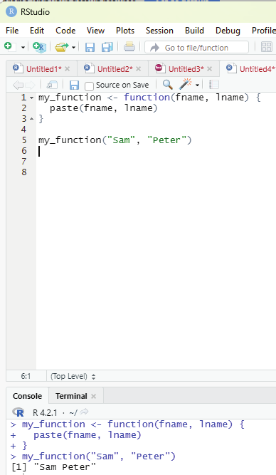

Image showing a function with two arguments
R Programming in Statistics


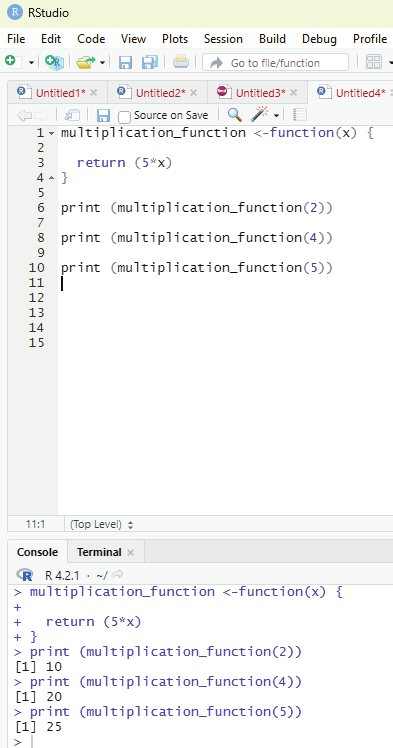

Image showing multiplication function
Prof. Dr Balasubramanian Thiagarajan
193


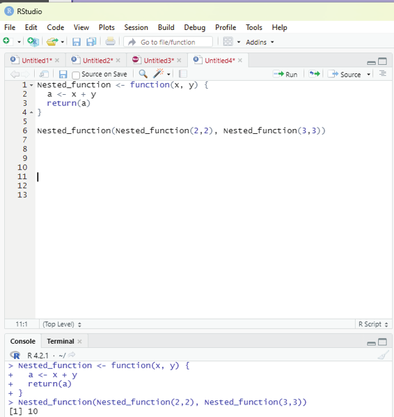

Image showing Nested function
R Programming in Statistics
The function instructs x to add y.
The first Nested_function(2,2) is “x” of the main function.
The input Nested_function(3,3) is “y” of the main function.
The output hence is (2+2) + (3+3) = 10
Recursion:
R accepts function recursion, which means a defined function can call itself. This is a common mathematical and programming concept. It means that a function cal s itself. This has the benefit of meaning that one can loop through data to reach a result.
The user should be careful with recursion function as it could easily slip into writing a function which never terminates thereby using excess amounts of memory or process power. Written correctly, it can be an efficient and mathematical y elegant programming practice.
Example:
recursion <- function(k) {
if (k>0) {
result <- k+recursion(k-1)
print(result)
} else {
result = 0
return(result)
}}
recursion(6)
R Global variables in functions:
Variables that are created outside of a function are known as global variables.
Example of creating a variable of a function and using it inside the function: txt <- “very good”
new_function <-function() {
paste(“R is”, txt)
}
new_function()
If the user tries to print txt, it will return the global variable which happens to be “very good”.
txt # print txt
Prof. Dr Balasubramanian Thiagarajan
195


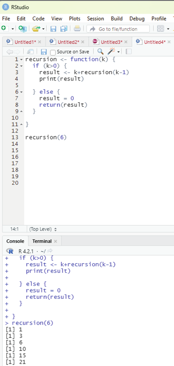

Image showing code for regression
R Programming in Statistics
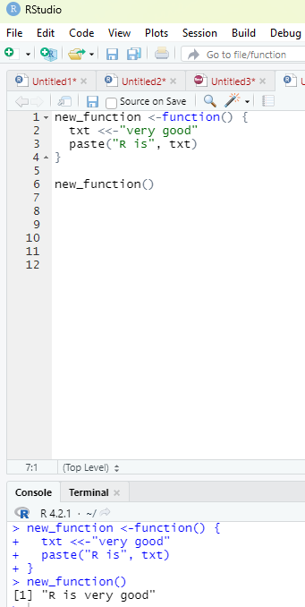
Normal y, when one wants to create a variable inside a function, that variable is local and can only be used inside that function. To create a global variable inside a function, one can use the global assignment operator
<<-
new_function <-function() {
txt <<-”very good”
paste(“R is”, txt)
}
new_function()
print(txt)
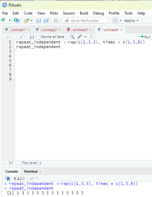
Repeat rep() function:
code:
repeat_eachnumber <-rep(c(1,2,3,4), each =4)
repeat_eachnumber
Repeat the sequence of the vector:
repeat_times <-rep(c(1,3,4,5), times =4)
repeat_times
Repeating each value independently:
repeat_independent <-rep(c(1,3,5), times = c(1,5,8)) repeat_independent
Prof. Dr Balasubramanian Thiagarajan
197
Image showing global assignment operator function
R Programming in Statistics


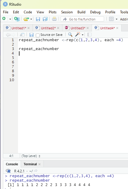

Image showing repeat function
Prof. Dr Balasubramanian Thiagarajan
199
Image showing each value being repeated independently
R Programming in Statistics