In this chapter, you will learn to:
Solve strictly determined games.
Solve games involving mixed strategies.
Game theory is one of the newest branches of mathematics. It first came to light when a brilliant mathematician named Dr. John von Neumann co-authored with Dr. Morgenstern a book titled Theory of Games and Economic Behavior. Since then it has played an important role in decision making in business, economics, social sciences and other fields.
In this chapter, we will study games that involve only two players. In these games, since a win for one person is a loss for the other, we refer to them as two-person zero-sum games. Although the games we will study here are fairly simple, they will provide us with an understanding of how games work and how they are applied in practical situations. We begin with an example.
Robert and Carol decide to play a game using a dime and a quarter. Each chooses one of the two coins, puts it in their hand and closes their fist. At a given signal, they simultaneously open their fists. If the sum of the coins is less than thirty five cents, Robert gets both coins, otherwise, Carol gets both coins. Write the matrix for the game, determine the optimal strategies for each player, and find the expected payoff for Robert.
Suppose Robert is the row player, that is, he plays the rows, and Carol is a column player. If Robert shows a dime and Carol shows a dime, the sum will be less than thirty five cents and Robert will win ten cents. But, if Robert shows a dime and Carol shows a quarter, the sum will not be less than thirty five cents and Carol will win ten cents or Robert will lose ten cents. The following matrix depicts all four cases and their corresponding payoffs for Robert. Remember a negative value is a loss for Robert and a win for Carol.

The best strategy for Robert is to always show a dime because this way the worst he can do is lose ten cents. And, the best strategy for Carol is to always show a quarter because that way the worst she can do is to lose ten cents. If both Robert and Carol play their optimal strategies, Robert will lose ten cents each time. Therefore, the value of the game is negative ten cents.
In Example 19.1, since there is only one fixed optimal strategy for each player, regardless of their opponent's strategy, we say the game possesses a pure strategy and is strictly determined.
Next, we formulate a method to find the optimal strategy for each player and the value of the game. The method involves considering the worst scenario for each player.
To consider the worst situation, the row player considers the minimum value in each row, and the column player considers the maximum value in each column. Note that the maximum value really represents a minimum value for the column player because the game matrix depicts the payoffs for the row player. We list the method below.
Put an asterisk(*) next to the minimum entry in each row.
Put a box around the maximum entry in each column.
The entry that has both an asterisk and a box represents the value of the game and is called a saddle point.
The row that is associated with the saddle point represents the best strategy for the row player, and the column that is associated with the saddle point represents the best strategy for the column player.
A game matrix can have more than one saddle point, but all saddle points have the same value.
If no saddle point exists, the game is not strictly determined. Non-strictly determined games are the subject of the section called “Non-Strictly Determined Games”.
Find the saddle points and optimal strategies for the following game.
We find the saddle point by placing an asterisk next to the minimum entry in each row, and by putting a box around the maximum entry in each column as shown below.
Since the second row, first column entry, which happens to be 10, has both an asterisk and a box, it is a saddle point. This implies that the value of the game is 10, and the optimal strategy for the row player is to always play row 2, and the optimal strategy for the column player is to always play column 1. If both players play their optimal strategies, the row player will win 10 units each time.
The row player's strategy is written as  indicating that he will play row 1 with a probability of 0 and row 2 with a probability of 1. Similarly the column player's strategy is
written as
indicating that he will play row 1 with a probability of 0 and row 2 with a probability of 1. Similarly the column player's strategy is
written as  implying that he will play column 1 with a probability of 1, and column 2 with a probability of 0.
In this section, we study games that have no saddle points. Which means that these games do not possess a pure strategy. We call these games non-strictly determined games. If the game is played only once, it will make no difference what move is made. However, if the game is played repeatedly, a mixed strategy consisting of alternating random moves can be worked out.
We consider the following example.
Suppose Robert and Carol decide to play a game using a dime and a quarter. At a given signal, they simultaneously show one of the two coins. If the coins match, Robert gets both coins, but if they don't match, Carol gets both coins. Determine whether the game is strictly determined.
We write the payoff matrix for Robert as follows:

To determine whether the game is strictly determined, we look for a saddle point. Again, we place an asterisk next to the minimum value in each row, and a box around the maximum value in each column. We get

Since there is no entry that has both an asterisk and a box, the game does not have a saddle point, and thus it is non-strictly determined.
We wish to devise a strategy for Robert. If Robert consistently shows a dime, for example, Carol will see the pattern and will start showing a quarter, and Robert will lose. Conversely, if Carol repeatedly shows a quarter, Robert will start showing a quarter, thus resulting in Carol's loss. So a good strategy is to throw your opponent off by showing a dime some of the times and showing a quarter other times. Before we develop an optimal strategy for each player, we will consider an arbitrary strategy for each and determine the corresponding payoffs.
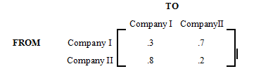
Suppose in Example 19.3, Robert decides to show a dime with .20 probability and a quarter with .80 probability, and Carol decides to show a dime with .70 probability and a quarter with .30 probability. What is the expected payoff for Robert?
Let R denote Robert's strategy and C denote Carol's strategy.
Since Robert is a row player and Carol is a column player, their strategies are written as follows:
 and
and
 .
.
To find the expected payoff, we use the following reasoning.
Since Robert chooses to play row 1 with .20 probability and Carol chooses to play column 1 with .70 probability, the move row 1, column 1 will be chosen with (.20)(.70)=.14 probability. The fact that this move has a payoff of 10 cents for Robert, Robert's expected payoff for this move is (.14)(.10)=.014 cents. Similarly, we compute Robert's expected payoffs for the other cases. The table below lists expected payoffs for all four cases.
| Move | Probability | Payoff | Expected Payoff |
| Row 1, Column 1 | ( . 20 ) ( . 70 ) = . 14 | 10 cents | 1.4 cents |
| Row 1, Column 2 | ( . 20 ) ( . 30 ) = . 06 | -10 cents | -.6 cents |
| Row 2, Column 1 | ( . 80 ) ( . 70 ) = . 56 | -25 cents | -14 cents |
| Row 2, Column 2 | ( . 80 ) ( . 30 ) = . 24 | 25 cents | 6.0 cents |
| Totals | 1 | -7.2 cents |
The above table shows that if Robert plays the game with the strategy
 and Carol plays with the strategy
 , Robert can expect to lose 7.2 cents for every game.
Alternatively, if we call the game matrix G, then the expected payoff for the row player can be determined by multiplying matrices R, G and C. Thus, the expected payoff P for Robert is as follows:

Which is the same as the one obtained from the table.
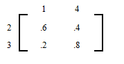
For the following game matrix G, determine the optimal strategy for both the row player and the column player, and find the value of the game.

Let us suppose that the row player uses the strategy
 . Now if the column player plays column 1, the expected payoff
P for the row player is
. Now if the column player plays column 1, the expected payoff
P for the row player is
P(r)=1(r)+(−3)(1−r)=4r−3.
Which can also be computed as follows:
 or
4r−3.
or
4r−3.
If the row player plays the strategy
 and the column player plays column 2, the expected payoff
P for the row player is
and the column player plays column 2, the expected payoff
P for the row player is
 .
.
We have two equations
P(r)=4r−3 and P(r)=−6r+4
The row player is trying to improve upon his worst scenario, and that only happens when the two lines intersect. Any point other than the point of intersection will not result in optimal strategy as one of the expectations will fall short.
Solving for r algebraically, we get
r=7/10.
Therefore, the optimal strategy for the row player is
 .
.
Alternatively, we can find the optimal strategy for the row player by, first, multiplying the row matrix with the game matrix as shown below.

And then by equating the two entries in the product matrix. Again, we get
r=.7, which gives us the optimal strategy
 .
.
We use the same technique to find the optimal strategy for the column player.
Suppose the column player's optimal strategy is represented by
 . We, first, multiply the game matrix by the column matrix as shown below.

And then equate the entries in the product matrix. We get
Therefore, the column player's optimal strategy is
 .
.
To find the expected value, V, of the game, we find the product of the matrices R, G and C.

That is, if both players play their optimal strategies, the row player can expect to lose .2 units for every game.
For the game in Example 19.3, determine the optimal strategy for both Robert and Carol, and find the value of the game.