Chapter 10. Multiple Regression: Part II

This chapter is published by NCPEA Press and is presented as an NCPEA/Connexions publication "print on demand book." Each chapter has been peer-reviewed, accepted, and endorsed by the National Council of Professors of Educational Administration (NCPEA) as a significant contribution to the scholarship and practice of education administration.
| John R. Slate is a Professor at Sam Houston State University where he teaches Basic and Advanced Statistics courses, as well as professional writing, to doctoral students in Educational Leadership and Counseling. His research interests lie in the use of educational databases, both state and national, to reform school practices. To date, he has chaired and/or served over 100 doctoral student dissertation committees. Recently, Dr. Slate created a website (Writing and Statistical Help) to assist students and faculty with both statistical assistance and in editing/writing their dissertations/theses and manuscripts. |
| Ana Rojas-LeBouef is a Literacy Specialist at the Reading Center at Sam Houston State University where she teaches developmental reading courses. Dr. LeBoeuf recently completed her doctoral degree in Reading, where she conducted a 16-year analysis of Texas statewide data regarding the achievement gap. Her research interests lie in examining the inequities in achievement among ethnic groups. Dr. Rojas-LeBouef also assists students and faculty in their writing and statistical needs on the Writing and Statistical Help website.
|
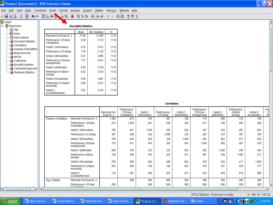
The first table in your SPSS output file should be a Descriptive Statistics table. You will see a column for M, SD, and n. This information should be used in your Results section.

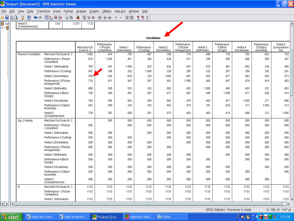
Underneath the Descriptive Statistics table is a table labeled Correlations. This table reflects the Pearson rs for each independent variable with the dependent variable, as well as the interrelationships among all of the variables.
Of the relationships of the independent variable with the Wechsler Full Scale IQ 3 (the dependent variable in this example), Verbal 2 (Similarities) has the highest correlation, .768. In a stepwise regression procedure, this variable should be the first statistically significant predictor.

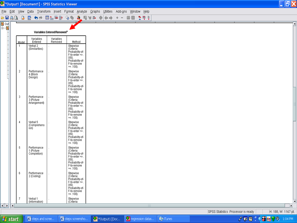
Next, you will see the Variables Entered/Removed table. We will not use the information in this table.

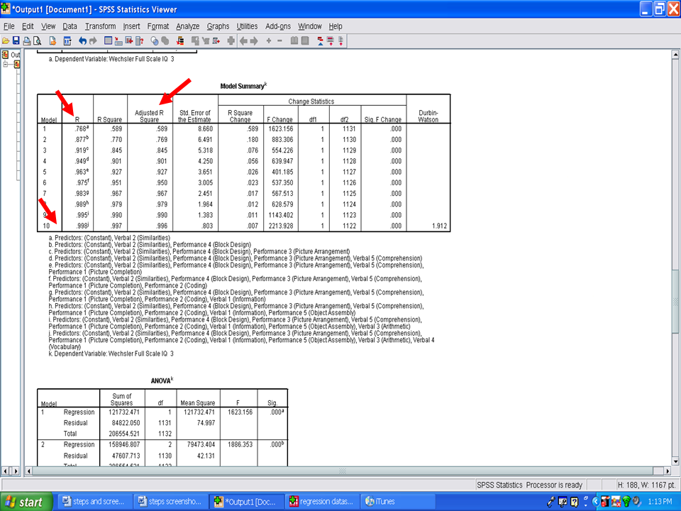
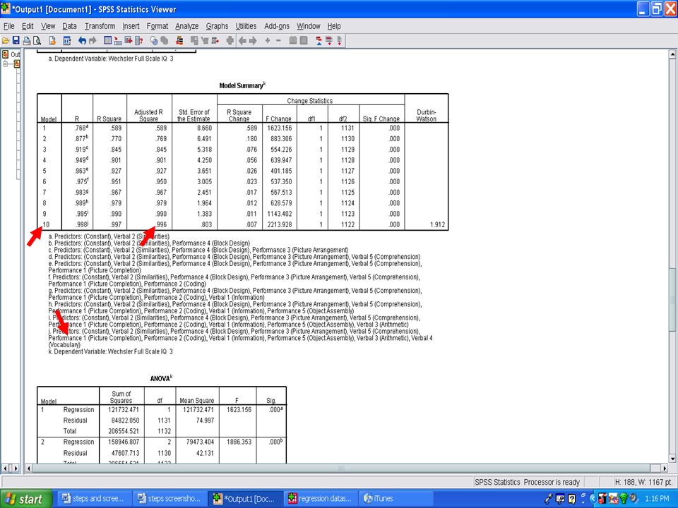
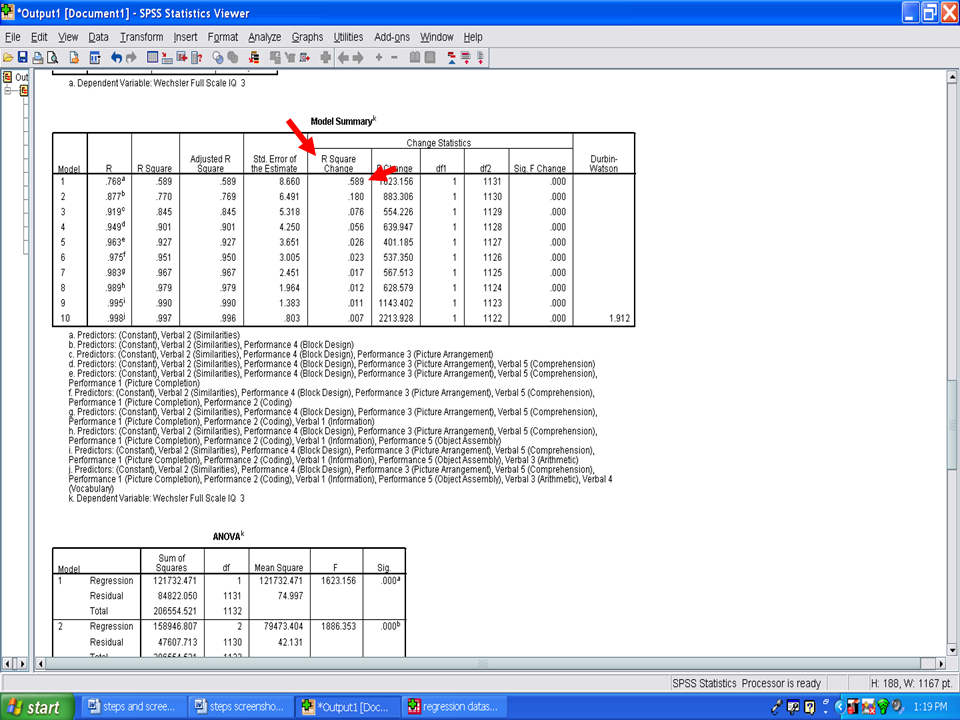
The table labeled Model Summary is an important table. This table is a summary of all of the steps entered/removed. Important columns in this table are:
Adjusted R Square
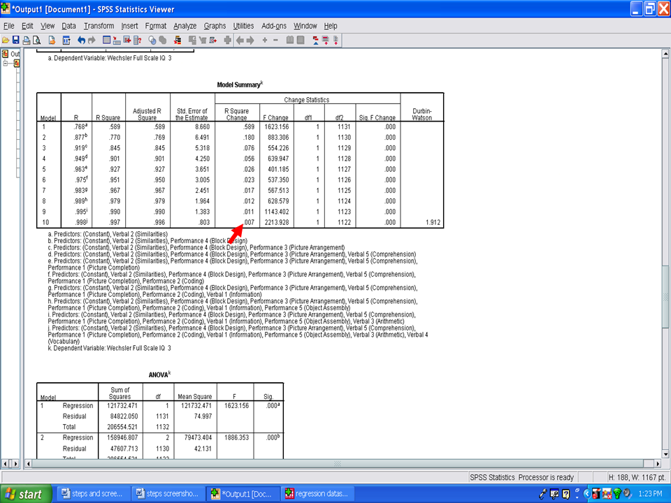
R Square Change
Durbin-Watson

The Durbin-Watson statistic is a measure for significant residual autocorrelation. Ideally it should be close to 2. In our example, the Durbin-Watson statistic is 1.912. Therefore, this assumption has not been violated.

The Adjusted R Square column indicates the amount of variance that each model explains in the dependent variable (i.e., Wechsler Fll Scale IQ 3). The first model has the letter a next to it. This model contains a single independent variable, Verbal 2 (Similarities). If you recall, this variable has the highest Pearson r with the Wechsler Full Scale IQ 3. In this example, Verbal 2 (Similarities) accounts for 58.9% of the variance in the Wechsler Full Scale IQ 3.

Each model, from 1 to 10, depicts the addition of another statistically significant variable in predicting the Wechsler Full Scale IQ 3. The final model, 10, indicates that all 10 independent variables accounted for 99.6% of the variance in the Wechsler Full Scale IQ 3.

Next, examine the R Square Change column. Each value reflects the unique variance in the Wechsler Full Scale IQ 3 explained by each statistically significant predictor variable. For Model 1, Verbal 2 (Similarities) explained the most variance, 58.9%. In Model 2, Performance 4 (Block Design) added 18.0% of unique variance that it explained.

The final model, 10, only added 0.7% of additional variance explained.

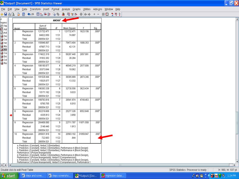
The next table of importance is the ANOVA table. Each model is examined to determine the extent to which it explains a statistically significant amount of the variance in the dependent variable. Of interest to us is the very last model, 10, which shows a statistically significant result, F(10, 1122) = 31959.947, p < .001.

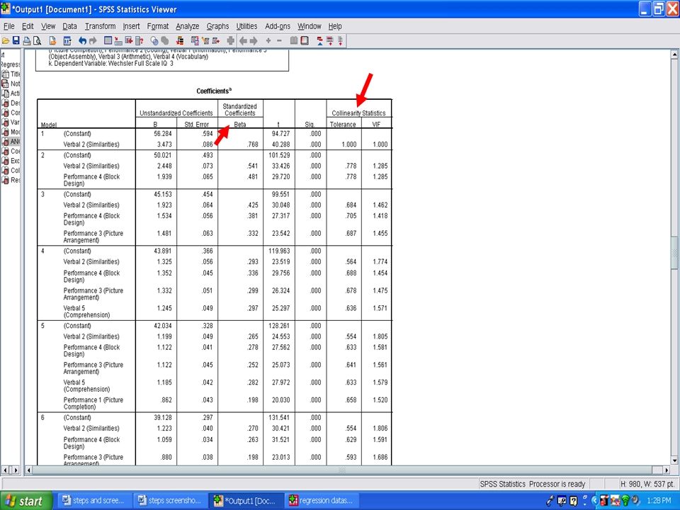
Underneath the ANOVA table is the Coefficients table. The important columns in this table are the Standardized Coefficients Beta and the Collinearity Statistics Tolerance and VIF ones. We will scroll down this table until we get to the final model, 10, information.

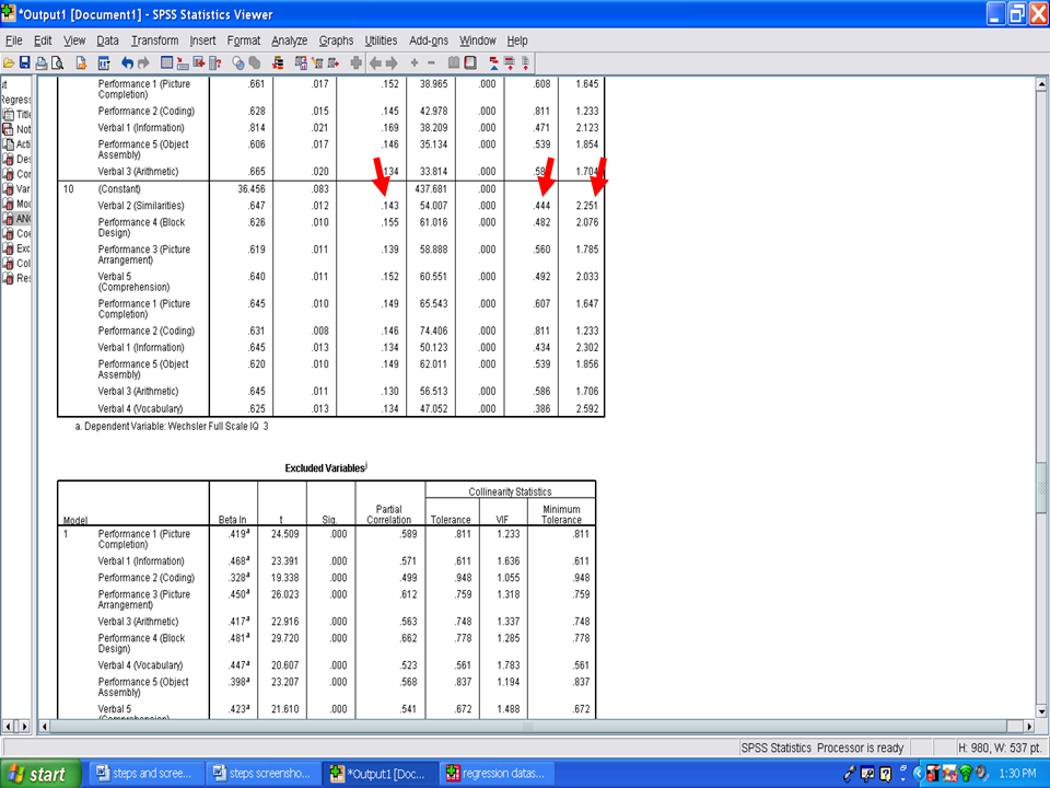
Scrolling down to the last model information shows us the following information. If you recall from the assumption checks, that multicollinearity was to be examined in the SPSS output. Multicollinearity is present when Tolerance values are below .1. As you can tell from the output below, Tolerance values range from a low of .386 to a high of .811. A second check for multicollinearity is the VIF column. Multicollinearity is present in the VIF column when the VIF values are greater than 10. In the example below, the VIF values range from a low of 1.233 to a high of 2.592. Therefore, multicollinearity is not present in this example.

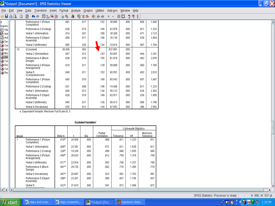
The Standardized Coefficients Beta column is to be examined next. Each of these values reflects the relative importance of each of these statistically significant predictors. In this column, you will see that the Betas range from a low of .130 to a high of .155, indicating that each has about the same degree of relative importance.

In your Results section, you should discuss the assumptions that you checked; the extent to which each assumption was met or not met; the descriptive statistics; and the information in the columns that was discussed at each step of the regression process.
You have now successfully gone through the calculation of a multiple regression analysis.


