Chapter 4. Discriminant Analysis: Assumptions

This chapter is published by NCPEA Press and is presented as an NCPEA/Connexions publication "print on demand book." Each chapter has been peer-reviewed, accepted, and endorsed by the National Council of Professors of Educational Administration (NCPEA) as a significant contribution to the scholarship and practice of education administration.
| John R. Slate is a Professor at Sam Houston State University where he teaches Basic and Advanced Statistics courses, as well as professional writing, to doctoral students in Educational Leadership and Counseling. His research interests lie in the use of educational databases, both state and national, to reform school practices. To date, he has chaired and/or served over 100 doctoral student dissertation committees. Recently, Dr. Slate created a website (Writing and Statistical Help) to assist students and faculty with both statistical assistance and in editing/writing their dissertations/theses and manuscripts. |
| Ana Rojas-LeBouef is a Literacy Specialist at the Reading Center at Sam Houston State University where she teaches developmental reading courses. Dr. LeBoeuf recently completed her doctoral degree in Reading, where she conducted a 16-year analysis of Texas statewide data regarding the achievement gap. Her research interests lie in examining the inequities in achievement among ethnic groups. Dr. Rojas-LeBouef also assists students and faculty in their writing and statistical needs on the Writing and Statistical Help website.
|
In this set of steps, readers will learn how to conduct a canonical discriminant analysis procedure. For detailed information regarding the assumptions underlying use of a discriminant analysis, readers are referred to the Hyperstats Online Statistics Textbook at http://davidmlane.com/hyperstat/ ; to the Electronic Statistics Textbook (2011) at http://www.statsoft.com/textbook/ ; or to Andy Field’s (2009) Discovering Statistics Using SPSS at http://www.amazon.com/Discovering-Statistics-Introducing-Statistical-Method/dp/1847879071/ref=sr_1_1?s=books&ie=UTF8&qid=1304967862&sr=1-1
Research questions for which a discriminant analysis procedure is appropriate involve determining variables that predict group membership. For example, if two groups of persons are present such as completers and non-completers and archival data are available, then a discriminant analysis procedure could be utilized. Such a procedure could identify specific variables that differentiate group membership. As such, interventions could be developed and targeted toward the variables that predicted group membership. Other sample research questions for which a discriminant analysis might be appropriate: (a) What factors differentiates successful from unsuccessful students?; (b) What factors differentiate delinquents from nondelinquents?; (c) What set of test scores best differentiates students with LD, students who are failing, and students with MR?; and (d) What set of factors differentiates drop-outs from persisters?
For purposes of this chapter, our research question is: “What scholastic variables differentiate boys from girls?”
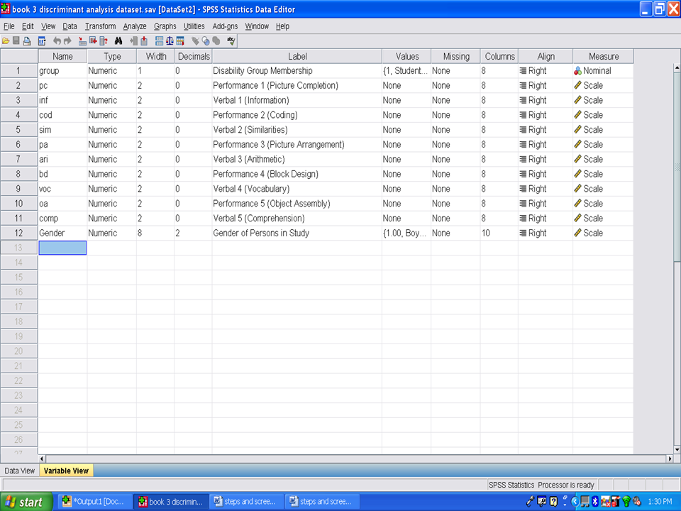
First, open up the dataset you intend to analyze for your canonical discriminant analysis.

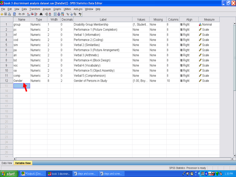
Our independent variable is gender. Boys are labeled as group 1 and girls are labeled as group 2.

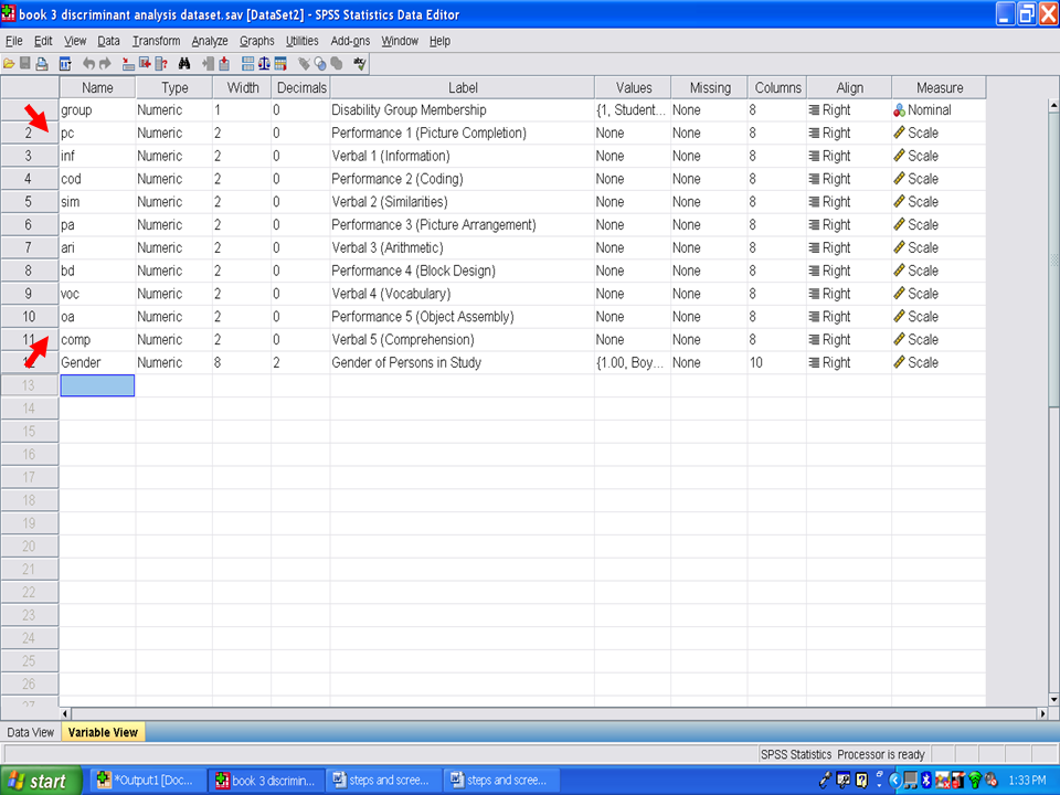
Our dependent variables, the ones we will use to differentiate boys from girls are 10 subscales from the Wechsler Intelligence Scale for Children-Third Edition: Picture Completion (pc), Information (inf), Coding (cod), Similarities (sim), Picture Arrangement (pa), Arithmetic (ari), Block Design (bd), Vocabulary (voc), Object Assembly (oa), and Comprehension (comp).

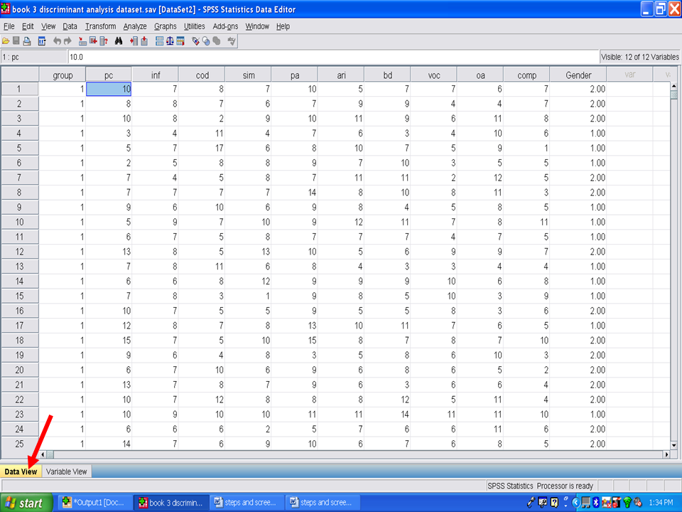
In the previous screenshots, we were in the variable view screen. Click on data view, shown below, so that your screen looks like the one below.

Prior to conducting a canonical discriminant function, we need to check the assumptions that underlie its use.
It is assumed that the data (for the variables) represent a sample from a multivariate normal distribution. You can examine whether or not variables are normally distributed with histograms of frequency distributions. However, note that violations of the normality assumption are usually not "fatal," meaning, that the resultant significance tests etc. are still "trustworthy." You may use specific tests for normality in addition to graphs. http://www.statsoft.com/textbook/discriminant-function-analysis/#assumptions
We recommend that you calculate the standardized skewness coefficients and the standardized kurtosis coefficients, as discussed in other chapters.
* Skewness [Note. Skewness refers to the extent to which the data are normally distributed around the mean. Skewed data involve having either mostly high scores with a few low ones or having mostly low scores with a few high ones.] Readers are referred to the following sources for a more detailed definition of skewness: http://www.statistics.com/index.php?page=glossary&term_id=356 and http://www.statsoft.com/textbook/basic-statistics/#Descriptive%20statisticsb
To standardize the skewness value so that its value can be constant across datasets and across studies, the following calculation must be made: Take the skewness value from the SPSS output and divide it by the Std. error of skewness. If the resulting calculation is within -3 to +3, then the skewness of the dataset is within the range of normality (Onwuegbuzie & Daniel, 2002). If the resulting calculation is outside of this +/-3 range, the dataset is not normally distributed.
* Kurtosis [Note. Kurtosis also refers to the extent to which the data are normally distributed around the mean. This time, the data are piled up higher than normal around the mean or piled up higher than normal at the ends of the distribution.] Readers are referred to the following sources for a more detailed definition of kurtosis: http://www.statistics.com/index.php?page=glossary&term_id=326 and http://www.statsoft.com/textbook/basic-statistics/#Descriptive%20statisticsb
To standardize the kurtosis value so that its value can be constant across datasets and across studies, the following calculation must be made: Take the kurtosis value from the SPSS output and divide it by the Std. error of kurtosis. If the resulting calculation is within -3 to +3, then the kurtosis of the dataset is within the range of normality (Onwuegbuzie & Daniel, 2002). If the resulting calculation is outside of this +/-3 range, the dataset is not normally distributed.
Correlations between Means and Variances
The major "real" threat to the validity of significance tests occurs when the means for variables across groups are correlated with the variances (or standard deviations). Intuitively, if there is large variability in a group with particularly high means on some variables, then those high means are not reliable. However, the overall significance tests are based on pooled variances, that is, the average variance across all groups. Thus, the significance tests of the relatively larger means (with the large variances) would be based on the relatively smaller pooled variances, resulting erroneously in statistical significance. In practice, this pattern may occur if one group in the study contains a few extreme outliers, who have a large impact on the means, and also increase the variability. To guard against this problem, inspect the descriptive statistics, that is, the means and standard deviations or variances for such a correlation. http://www.statsoft.com/textbook/discriminant-function-analysis/#assumptions
After calculating the means and standard deviations for your variables for each of your groups, check them to determine if large variability is present in the means for one of your groups compared to the means for the other group.
The Matrix Ill-Conditioning Problem
Another assumption of discriminant function analysis is that the variables that are used to discriminate between groups are not completely redundant. As part of the computations involved in discriminant analysis, you will invert the variance/covariance matrix of the variables in the model. If any one of the variables is completely redundant with the other variables then the matrix is said to be ill-conditioned, and it cannot be inverted. For example, if a variable is the sum of three other variables that are also in the model, then the matrix is ill-conditioned. http://www.statsoft.com/textbook/discriminant-function-analysis/#assumptions
What this assumption means is that each variable should be unique from any other variable in the analysis. Having one variable that includes another variable would be a violation of this assumption. An example of this would be using a total score that contains several subscale scores, all of which are used in the discriminant analysis.
In order to guard against matrix ill-conditioning, constantly check the so-called tolerance value for each variable. This tolerance value is computed as 1 minus R-square of the respective variable with all other variables included in the current model. Thus, it is the proportion of variance that is unique to the respective variable. In general, when a variable is almost completely redundant (and, therefore, the matrix ill-conditioning problem is likely to occur), the tolerance value for that variable will approach 0. http://www.statsoft.com/textbook/discriminant-function-analysis/#assumptions
We will check this assumption, the tolerance values, when we examine the SPSS output.


