5.1 Discrete Random Variables1
5.1.1 Student Learning Outcomes
By the end of this chapter, the student should be able to:
• Recognize and understand discrete probability distribution functions, in general.
• Calculate and interpret expected values.
• Recognize the binomial probability distribution and apply it appropriately.
• Recognize the Poisson probability distribution and apply it appropriately (optional).
• Recognize the geometric probability distribution and apply it appropriately (optional).
• Recognize the hypergeometric probability distribution and apply it appropriately (optional).
• Classify discrete word problems by their distributions.
5.1.2 Introduction
A student takes a 10 question true-false quiz. Because the student had such a busy schedule, he or she
could not study and randomly guesses at each answer. What is the probability of the student passing the
test with at least a 70%?
Small companies might be interested in the number of long distance phone calls their employees make
during the peak time of the day. Suppose the average is 20 calls. What is the probability that the employees
make more than 20 long distance phone calls during the peak time?
These two examples illustrate two different types of probability problems involving discrete random vari-
ables. Recall that discrete data are data that you can count. A random variable describes the outcomes
of a statistical experiment in words. The values of a random variable can vary with each repetition of an
experiment.
In this chapter, you will study probability problems involving discrete random distributions. You will also
study long-term averages associated with them.
5.1.3 Random Variable Notation
Upper case letters like X or Y denote a random variable. Lower case letters like x or y denote the value of a
random variable. If X is a random variable, then X is written in words. and x is given as a number.
1This content is available online at <http://cnx.org/content/m16825/1.14/>.
209
210
CHAPTER 5. DISCRETE RANDOM VARIABLES
For example, let X = the number of heads you get when you toss three fair coins. The sample space for the
toss of three fair coins is TTT; THH; HTH; HHT; HTT; THT; TTH; HHH. Then, x = 0, 1, 2, 3. X is in
words and x is a number. Notice that for this example, the x values are countable outcomes. Because you
can count the possible values that X can take on and the outcomes are random (the x values 0, 1, 2, 3), X is
a discrete random variable.
5.1.4 Optional Collaborative Classroom Activity
Toss a coin 10 times and record the number of heads. After all members of the class have completed the
experiment (tossed a coin 10 times and counted the number of heads), fill in the chart using a heading like
the one below. Let X = the number of heads in 10 tosses of the coin.
x
Frequency of x
Relative Frequency of x
Table 5.1
• Which value(s) of x occurred most frequently?
• If you tossed the coin 1,000 times, what values could x take on? Which value(s) of x do you think
would occur most frequently?
• What does the relative frequency column sum to?
5.2 Probability Distribution Function (PDF) for a Discrete Random
Variable2
A discrete probability distribution function has two characteristics:
• Each probability is between 0 and 1, inclusive.
• The sum of the probabilities is 1.
Example 5.1
A child psychologist is interested in the number of times a newborn baby’s crying wakes its mother
after midnight. For a random sample of 50 mothers, the following information was obtained. Let
X = the number of times a newborn wakes its mother after midnight. For this example, x = 0, 1, 2,
3, 4, 5.
P(x) = probability that X takes on a value x.
2This content is available online at <http://cnx.org/content/m16831/1.14/>.
211
x
P(x)
0
P(x=0) = 2
50
1
P(x=1) = 11
50
2
P(x=2) = 23
50
3
P(x=3) = 9
50
4
P(x=4) = 4
50
5
P(x=5) = 1
50
Table 5.2
X takes on the values 0, 1, 2, 3, 4, 5. This is a discrete PDF because
1. Each P(x) is between 0 and 1, inclusive.
2. The sum of the probabilities is 1, that is,
2
11
23
9
4
1
+
+
+
+
+
= 1
(5.1)
50
50
50
50
50
50
Example 5.2
Suppose Nancy has classes 3 days a week. She attends classes 3 days a week 80% of the time, 2
days 15% of the time, 1 day 4% of the time, and no days 1% of the time. Suppose one week is
randomly selected.
Problem 1
(Solution on p. 244.)
Let X = the number of days Nancy ____________________ .
Problem 2
(Solution on p. 244.)
X takes on what values?
Problem 3
(Solution on p. 244.)
Suppose one week is randomly chosen. Construct a probability distribution table (called a PDF
table) like the one in the previous example. The table should have two columns labeled x and P(x).
What does the P(x) column sum to?
5.3 Mean or Expected Value and Standard Deviation3
The expected value is often referred to as the "long-term"average or mean . This means that over the long
term of doing an experiment over and over, you would expect this average.
The mean of a random variable X is µ. If we do an experiment many times (for instance, flip a fair coin, as
Karl Pearson did, 24,000 times and let X = the number of heads) and record the value of X each time, the
average is likely to get closer and closer to µ as we keep repeating the experiment. This is known as the
Law of Large Numbers.
NOTE: To find the expected value or long term average, µ, simply multiply each value of the
random variable by its probability and add the products.
3This content is available online at <http://cnx.org/content/m16828/1.16/>.
212
CHAPTER 5. DISCRETE RANDOM VARIABLES
A Step-by-Step Example
A men’s soccer team plays soccer 0, 1, or 2 days a week. The probability that they play 0 days is 0.2, the
probability that they play 1 day is 0.5, and the probability that they play 2 days is 0.3. Find the long-term
average, µ, or expected value of the days per week the men’s soccer team plays soccer.
To do the problem, first let the random variable X = the number of days the men’s soccer team plays soccer
per week. X takes on the values 0, 1, 2. Construct a PDF table, adding a column xP (x). In this column,
you will multiply each x value by its probability.
Expected Value Table
x
P(x)
xP(x)
0
0.2
(0)(0.2) = 0
1
0.5
(1)(0.5) = 0.5
2
0.3
(2)(0.3) = 0.6
Table 5.4: This table is called an expected value table. The table helps you calculate the expected value or
long-term average.
Add
the
last
column
to
find
the
long
term
average
or
expected
value:
(0) (0.2) + (1) (0.5) + (2) (0.3) = 0 + 0.5 + 0.6 = 1.1.
The expected value is 1.1. The men’s soccer team would, on the average, expect to play soccer 1.1 days
per week. The number 1.1 is the long term average or expected value if the men’s soccer team plays soccer
week after week after week. We say µ = 1.1
Example 5.3
Find the expected value for the example about the number of times a newborn baby’s crying
wakes its mother after midnight. The expected value is the expected number of times a newborn
wakes its mother after midnight.
x
P(X)
xP(X)
0
P(x=0) = 2
(0) 2
= 0
50
50
1
P(x=1) = 11
(1) 11 = 11
50
50
50
2
P(x=2) = 23
(2) 23 = 46
50
50
50
3
P(x=3) = 9
(3) 9
= 27
50
50
50
4
P(x=4) = 4
(4) 4
= 16
50
50
50
5
P(x=5) = 1
(5) 1
= 5
50
50
50
Table 5.5: You expect a newborn to wake its mother after midnight 2.1 times, on the average.
Add the last column to find the expected value. µ = Expected Value = 105 = 2.1
50
Problem
Go back and calculate the expected value for the number of days Nancy attends classes a week.
Construct the third column to do so.
Solution
2.74 days a week.
213
Example 5.4
Suppose you play a game of chance in which five numbers are chosen from 0, 1, 2, 3, 4, 5, 6, 7, 8,
9. A computer randomly selects five numbers from 0 to 9 with replacement. You pay $2 to play
and could profit $100,000 if you match all 5 numbers in order (you get your $2 back plus $100,000).
Over the long term, what is your expected profit of playing the game?
To do this problem, set up an expected value table for the amount of money you can profit.
Let X = the amount of money you profit. The values of x are not 0, 1, 2, 3, 4, 5, 6, 7, 8, 9. Since you
are interested in your profit (or loss), the values of x are 100,000 dollars and -2 dollars.
To win, you must get all 5 numbers correct, in order. The probability of choosing one correct
number is 1 because there are 10 numbers. You may choose a number more than once. The
10
probability of choosing all 5 numbers correctly and in order is:
1
1
1
1
1
∗
∗
∗
∗
∗ = 1 ∗ 10−5 = 0.00001
(5.2)
10
10
10
10
10
Therefore, the probability of winning is 0.00001 and the probability of losing is
1 − 0.00001 = 0.99999
(5.3)
The expected value table is as follows.
x
P(x)
xP(x)
Loss
-2
0.99999
(-2)(0.99999)=-1.99998
Profit
100,000
0.00001
(100000)(0.00001)=1
Table 5.6: Add the last column. -1.99998 + 1 = -0.99998
Since −0.99998 is about −1, you would, on the average, expect to lose approximately one dollar
for each game you play. However, each time you play, you either lose $2 or profit $100,000. The $1
is the average or expected LOSS per game after playing this game over and over.
Example 5.5
Suppose you play a game with a biased coin. You play each game by tossing the coin once.
P(heads) = 2 and P(tails) = 1 . If you toss a head, you pay $6. If you toss a tail, you win $10.
3
3
If you play this game many times, will you come out ahead?
Problem 1
(Solution on p. 244.)
Define a random variable X.
Problem 2
(Solution on p. 244.)
Complete the following expected value table.
x
____
____
WIN
10
1
____
3
LOSE
____
____
−12
3
Table 5.7
214
CHAPTER 5. DISCRETE RANDOM VARIABLES
Problem 3
(Solution on p. 244.)
What is the expected value, µ? Do you come out ahead?
Like data, probability distributions have standard deviations. To calculate the standard deviation ( σ) of a
probability distribution, find each deviation from its expected value, square it, multiply it by its probability,
add the products, and take the square root . To understand how to do the calculation, look at the table for
the number of days per week a men’s soccer team plays soccer. To find the standard deviation, add the
entries in the column labeled (x − µ)2 · P (x) and take the square root.
x
P(x)
xP(x)
(x - µ)2P(x)
0
0.2
(0)(0.2) = 0
(0 − 1.1)2 (.2) = 0.242
1
0.5
(1)(0.5) = 0.5
(1 − 1.1)2 (.5) = 0.005
2
0.3
(2)(0.3) = 0.6
(2 − 1.1)2 (.3) = 0.243
Table 5.8
Add the last column in the table. 0.242 + 0.005 + 0.243 = 0.490. The standard deviation is the square root
√
of 0.49. σ =
0.49 = 0.7
Generally for probability distributions, we use a calculator or a computer to calculate µ and σ to reduce
roundoff error. For some probability distributions, there are short-cut formulas that calculate µ and σ.
5.4 Common Discrete Probability Distribution Functions4
Some of the more common discrete probability functions are binomial, geometric, hypergeometric, and
Poisson. Most elementary courses do not cover the geometric, hypergeometric, and Poisson. Your instruc-
tor will let you know if he or she wishes to cover these distributions.
A probability distribution function is a pattern. You try to fit a probability problem into a pattern or distri-
bution in order to perform the necessary calculations. These distributions are tools to make solving prob-
ability problems easier. Each distribution has its own special characteristics. Learning the characteristics
enables you to distinguish among the different distributions.
5.5 Binomial5
The characteristics of a binomial experiment are:
1. There are a fixed number of trials. Think of trials as repetitions of an experiment. The letter n denotes
the number of trials.
2. There are only 2 possible outcomes, called "success" and, "failure" for each trial. The letter p denotes
the probability of a success on one trial and q denotes the probability of a failure on one trial. p + q = 1.
3. The n trials are independent and are repeated using identical conditions. Because the n trials are in-
dependent, the outcome of one trial does not help in predicting the outcome of another trial. Another
way of saying this is that for each individual trial, the probability, p, of a success and probability, q,
of a failure remain the same. For example, randomly guessing at a true - false statistics question has
only two outcomes. If a success is guessing correctly, then a failure is guessing incorrectly. Suppose
4This content is available online at <http://cnx.org/content/m16821/1.6/>.
5This content is available online at <http://cnx.org/content/m16820/1.16/>.
215
Joe always guesses correctly on any statistics true - false question with probability p = 0.6. Then,
q = 0.4 .This means that for every true - false statistics question Joe answers, his probability of success
(p = 0.6) and his probability of failure (q = 0.4) remain the same.
The outcomes of a binomial experiment fit a binomial probability distribution. The random variable X =
the number of successes obtained in the n independent trials.
The mean,
2
2
µ, and variance, σ , for the binomial probability distribution is µ = n p and σ
= npq. The
√
standard deviation, σ, is then σ =
npq.
Any experiment that has characteristics 2 and 3 and where n = 1 is called a Bernoulli Trial (named after
Jacob Bernoulli who, in the late 1600s, studied them extensively). A binomial experiment takes place when
the number of successes is counted in one or more Bernoulli Trials.
Example 5.6
At ABC College, the withdrawal rate from an elementary physics course is 30% for any given
term. This implies that, for any given term, 70% of the students stay in the class for the entire
term. A "success" could be defined as an individual who withdrew. The random variable is X =
the number of students who withdraw from the randomly selected elementary physics class.
Example 5.7
Suppose you play a game that you can only either win or lose. The probability that you win any
game is 55% and the probability that you lose is 45%. Each game you play is independent. If you
play the game 20 times, what is the probability that you win 15 of the 20 games? Here, if you
define X = the number of wins, then X takes on the values 0, 1, 2, 3, ..., 20. The probability of a
success is p = 0.55. The probability of a failure is q = 0.45. The number of trials is n = 20. The
probability question can be stated mathematically as P (x = 15).
Example 5.8
A fair coin is flipped 15 times. Each flip is independent. What is the probability of getting more
than 10 heads? Let X = the number of heads in 15 flips of the fair coin. X takes on the values 0, 1,
2, 3, ..., 15. Since the coin is fair, p = 0.5 and q = 0.5. The number of trials is n = 15. The probability
question can be stated mathematically as P (x > 10).
Example 5.9
Approximately 70% of statistics students do their homework in time for it to be collected and
graded. Each student does homework independently. In a statistics class of 50 students, what is
the probability that at least 40 will do their homework on time? Students are selected randomly.
Problem 1
(Solution on p. 244.)
This is a binomial problem because there is only a success or a __________, there are a definite
number of trials, and the probability of a success is 0.70 for each trial.
Problem 2
(Solution on p. 244.)
If we are interested in the number of students who do their homework, then how do we define
X?
Problem 3
(Solution on p. 244.)
What values does x take on?
Problem 4
(Solution on p. 244.)
What is a "failure", in words?
The probability of a success is p = 0.70. The number of trial is n = 50.
Problem 5
(Solution on p. 244.)
If p + q = 1, then what is q?
216
CHAPTER 5. DISCRETE RANDOM VARIABLES
Problem 6
(Solution on p. 244.)
The words "at least" translate as what kind of inequality for the probability question P (x____40).
The probability question is P (x ≥ 40).
5.5.1 Notation for the Binomial: B = Binomial Probability Distribution Function
X ∼ B (n, p)
Read this as "X is a random variable with a binomial distribution." The parameters are n and p. n = number
of trials p = probability of a success on each trial
Example 5.10
It has been stated that about 41% of adult workers have a high school diploma but do not pursue
any further education. If 20 adult workers are randomly selected, find the probability that at most
12 of them have a high school diploma but do not pursue any further education. How many adult
workers do you expect to have a high school diploma but do not pursue any further education?
Let X = the number of workers who have a high school diploma but do not pursue any further
education.
X takes on the values 0, 1, 2, ..., 20 where n = 20 and p = 0.41. q = 1 - 0.41 = 0.59. X ∼ B (20, 0.41)
Find P (x ≤ 12) . P (x ≤ 12) = 0.9738. (calculator or computer)
Using the TI-83+ or the TI-84 calculators, the calculations are as follows. Go into 2nd DISTR. The
syntax for the instructions are
To calculate (x = value): binompdf(n, p, number) If "number" is left out, the result is the binomial probability table.
To calculate P (x ≤ value): binomcdf(n, p, number) If "number" is left out, the result is the cumulative binomial probability table.
For this problem: After you are in 2nd DISTR, arrow down to A:binomcdf. Press ENTER. Enter
20,.41,12). The result is P (x ≤ 12) = 0.9738.
NOTE: If you want to find P (x = 12), use the pdf (0:binompdf). If you want to find P (x (> , 12)),
use 1 - binomcdf(20,.41,12).
The probability at most 12 workers have a high school diploma but do not pursue any further
education is 0.9738
The graph of x ∼ B (20, 0.41) is:
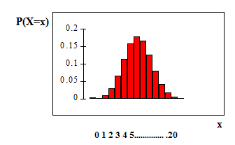
217
The y-axis contains the probability of x, where X = the number of workers who have only a high
school diploma.
The number of adult workers that you expect to have a high school diploma but not pursue any
further education is the mean, µ = np = (20) (0.41) = 8.2.
√
The formula for the variance is
2
σ
= npq.
The standard deviation is σ =
npq.
σ
=
(20) (0.41) (0.59) = 2.20.
Example 5.11
The following example illustrates a problem that is not binomial. It violates the condition of in-
dependence. ABC College has a student advisory committee made up of 10 staff members and
6 students. The committee wishes to choose a chairperson and a recorder. What is the proba-
bility that the chairperson and recorder are both students? All names of the committee are put
into a box and two names are drawn