EXAMPLES: Here are two examples, but you may NOT use them: height vs. weight and age
vs. running distance.
____ Describe how your group is going to collect the data (for instance, collect data from the web, survey
students on campus).
____ Describe your sampling technique in detail. Use cluster, stratified, systematic, or simple random
sampling (using a random number generator) sampling. Convenience sampling is NOT acceptable.
____ Conduct your survey. Your number of pairs must be at least 30.
____ Print out a copy of your data.
Analysis
____ On a separate sheet of paper construct a scatter plot of the data. Label and scale both axes.
____ State the least squares line and the correlation coefficient.
____ On your scatter plot, in a different color, construct the least squares line.
____ Is the correlation coefficient significant? Explain and show how you determined this.
____ Interpret the slope of the linear regression line in the context of the data in your project. Relate the
explanation to your data, and quantify what the slope tells you.
____ Does the regression line seem to fit the data? Why or why not? If the data does not seem to be linear,
explain if any other model seems to fit the data better.
____ Are there any outliers? If so, what are they? Show your work in how you used the potential outlier
formula in the Linear Regression and Correlation chapter (since you have bivariate data) to determine
whether or not any pairs might be outliers.
8This content is available online at <http://cnx.org/content/m17143/1.6/>.
APPENDIX
557
13.4.5.4 Part II: Univariate Data
In this section, you will use the data for ONE variable only. Pick the variable that is more interesting to
analyze. For example: if your independent variable is sequential data such as year with 30 years and one
piece of data per year, your x-values might be 1971, 1972, 1973, 1974, . . ., 2000. This would not be interesting
to analyze. In that case, choose to use the dependent variable to analyze for this part of the project.
_____ Summarize your data in a chart with columns showing data value, frequency, relative frequency,
and cumulative relative frequency.
_____ Answer the following, rounded to 2 decimal places:
1. Sample mean =
2. Sample standard deviation =
3. First quartile =
4. Third quartile =
5. Median =
6. 70th percentile =
7. Value that is 2 standard deviations above the mean =
8. Value that is 1.5 standard deviations below the mean =
_____ Construct a histogram displaying your data. Group your data into 6 – 10 intervals of equal width.
Pick regularly spaced intervals that make sense in relation to your data. For example, do NOT group
data by age as 20-26,27-33,34-40,41-47,48-54,55-61 . . . Instead, maybe use age groups 19.5-24.5, 24.5-
29.5, . . . or 19.5-29.5, 29.5-39.5, 39.5-49.5, . . .
_____ In complete sentences, describe the shape of your histogram.
_____ Are there any potential outliers? Which values are they? Show your work and calculations as to
how you used the potential outlier formula in chapter 2 (since you are now using univariate data) to
determine which values might be outliers.
_____ Construct a box plot of your data.
_____ Does the middle 50% of your data appear to be concentrated together or spread out? Explain how
you determined this.
_____ Looking at both the histogram AND the box plot, discuss the distribution of your data. For example:
how does the spread of the middle 50% of your data compare to the spread of the rest of the data rep-
resented in the box plot; how does this correspond to your description of the shape of the histogram;
how does the graphical display show any outliers you may have found; does the histogram show any
gaps in the data that are not visible in the box plot; are there any interesting features of your data that
you should point out.
13.4.5.5 Due Dates
• Part I, Intro: __________ (keep a copy for your records)
• Part I, Analysis: __________ (keep a copy for your records)
• Entire Project, typed and stapled: __________
____ Cover sheet: names, class time, and name of your study.
____ Part I: label the sections “Intro” and “Analysis.”
____ Part II:
____ Summary page containing several paragraphs written in complete sentences describing the ex-
periment, including what you studied and how you collected your data. The summary page
should also include answers to ALL the questions asked above.
____ All graphs requested in the project.
____ All calculations requested to support questions in data.
____ Description: what you learned by doing this project, what challenges you had, how you over-
came the challenges.
558
APPENDIX
NOTE:
Include answers to ALL questions asked, even if not explicitly repeated in the items
above.

APPENDIX
559
13.5 Solution Sheets
13.5.1 Solution Sheet: Hypothesis Testing for Single Mean and Single Proportion9
Class Time:
Name:
a. Ho:
b. Ha:
c. In words, CLEARLY state what your random variable X or P’ represents.
d. State the distribution to use for the test.
e. What is the test statistic?
f. What is the p-value? In 1 – 2 complete sentences, explain what the p-value means for this problem.
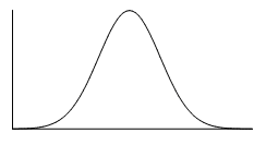
g. Use the previous information to sketch a picture of this situation. CLEARLY, label and scale the horizon-
tal axis and shade the region(s) corresponding to the p-value.
Figure 13.1
h. Indicate the correct decision (“reject” or “do not reject” the null hypothesis), the reason for it, and write
an appropriate conclusion, using complete sentences.
i. Alpha:
ii. Decision:
iii. Reason for decision:
iv. Conclusion:
i. Construct a 95% Confidence Interval for the true mean or proportion. Include a sketch of the graph of
the situation. Label the point estimate and the lower and upper bounds of the Confidence Interval.
Figure 13.2
9This content is available online at <http://cnx.org/content/m17134/1.6/>.

560
APPENDIX
13.5.2 Solution Sheet: Hypothesis Testing for Two Means, Paired Data, and Two
Proportions10
Class Time:
Name:
a. Ho: _______
b. Ha: _______
c. In words, clearly state what your random variable X1 − X2, P1’ − P2’- or Xd represents.
d. State the distribution to use for the test.
e. What is the test statistic?
f. What is the p-value? In 1 – 2 complete sentences, explain what the p-value means for this problem.
g. Use the previous information to sketch a picture of this situation. CLEARLY label and scale the horizon-
tal axis and shade the region(s) corresponding to the p-value.
Figure 13.3
h. Indicate the correct decision (“reject” or “do not reject” the null hypothesis), the reason for it, and write
an appropriate conclusion, using complete sentences.
i. Alpha:
ii. Decision:
iii. Reason for decision:
iv. Conclusion:
i. In complete sentences, explain how you determined which distribution to use.
10This content is available online at <http://cnx.org/content/m17133/1.6/>.
APPENDIX
561
13.5.3 Solution Sheet: The Chi-Square Distribution11
Class Time:
Name:
a. Ho: _______
b. Ha:
c. What are the degrees of freedom?
d. State the distribution to use for the test.
e. What is the test statistic?
f. What is the p-value? In 1 – 2 complete sentences, explain what the p-value means for this problem.
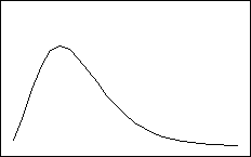
g. Use the previous information to sketch a picture of this situation. Clearly label and scale the horizontal
axis and shade the region(s) corresponding to the p-value.
Figure 13.4
h. Indicate the correct decision (“reject” or “do not reject” the null hypothesis) and write appropriate con-
clusions, using complete sentences.
i. Alpha:
ii. Decision:
iii. Reason for decision:
iv. Conclusion:
11This content is available online at <http://cnx.org/content/m17136/1.5/>.
562
APPENDIX
13.5.4 Solution Sheet: F Distribution and ANOVA12
Class Time:
Name:
a. Ho:
b. Ha:
c. df (n) =
d. df (d) =
e. State the distribution to use for the test.
f. What is the test statistic?
g. What is the p-value? In 1 – 2 complete sentences, explain what the p-value means for this problem.
h. Use the previous information to sketch a picture of this situation. Clearly label and scale the horizontal
axis and shade the region(s) corresponding to the p-value.
Figure 13.5
i. Indicate the correct decision (“reject” or “do not reject” the null hypothesis) and write appropriate con-
clusions, using complete sentences.
i. Alpha:
ii. Decision:
iii. Reason for decision:
iv. Conclusion:
12This content is available online at <http://cnx.org/content/m17135/1.5/>.
APPENDIX
563
13.6 English Phrases Written Mathematically13
13.6.1 English Phrases Written Mathematically
When the English says:
Interpret this as:
Xis at least 4.
X ≥ 4
XThe minimum is 4.
X ≥ 4
X is no less than 4.
X ≥ 4
X is greater than or equal to 4.
X ≥ 4
X is at most 4.
X ≤ 4
XThe maximum is 4.
X ≤ 4
Xis no more than 4.
X ≤ 4
X is less than or equal to 4.
X ≤ 4
Xdoes not exceed 4.
X ≤ 4
Xis greater than 4.
X > 4
XThere are more than 4.
X > 4
Xexceeds 4.
X > 4
Xis less than 4.
X < 4
XThere are fewer than 4.
X < 4
Xis 4.
X = 4
Xis equal to 4.
X = 4
Xis the same as 4.
X = 4
Xis not 4.
X = 4
Xis not equal to 4.
X = 4
Xis not the same as 4.
X = 4
Xis different than 4.
X = 4
Table 13.16
13This content is available online at <http://cnx.org/content/m16307/1.5/>.
564
APPENDIX
13.7 Symbols and their Meanings14
Symbols and their Meanings
Chapter (1st used)
Symbol
Spoken
Meaning
√
Sampling and Data
The square root of
same
Sampling and Data
π
Pi
3.14159. . . (a specific
number)
Descriptive Statistics
Q1
Quartile one
the first quartile
Descriptive Statistics
Q2
Quartile two
the second quartile
Descriptive Statistics
Q3
Quartile three
the third quartile
Descriptive Statistics
IQR
inter-quartile range
Q3-Q1=IQR
Descriptive Statistics
x
x-bar
sample mean
Descriptive Statistics
µ
mu
population mean
Descriptive Statistics
s sx sx
s
sample standard devia-
tion
Descriptive Statistics
s2 s2x
s-squared
sample variance
Descriptive Statistics
σ σ x σ x
sigma
population
standard
deviation
Descriptive Statistics
2
2
σ σ x
sigma-squared
population variance
Descriptive Statistics
Σ
capital sigma
sum
Probability Topics
{}
brackets
set notation
Probability Topics
S
S
sample space
Probability Topics
A
Event A
event A
Probability Topics
P (A)
probability of A
probability of A occur-
ring
Probability Topics
P (A | B)
probability of A given B
prob.
of A occurring
given B has occurred
Probability Topics
P (AorB)
prob. of A or B
prob. of A or B or both
occurring
continued on next page
14This content is available online at <http://cnx.org/content/m16302/1.9/>.
APPENDIX
565
Probability Topics
P (AandB)
prob. of A and B
prob. of both A and B
occurring (same time)
Probability Topics
A’
A-prime, complement
complement of A, not A
of A
Probability Topics
P (A’)
prob. of complement of
same
A
Probability Topics
G1
green on first pick
same
Probability Topics
P (G1)
prob. of green on first
same
pick
Discrete Random Vari-
prob. distribution func-
same
ables
tion
Discrete Random Vari-
X
X
the random variable X
ables
Discrete Random Vari-
X ∼
the distribution of X
same
ables
Discrete Random Vari-
B
binomial distribution
same
ables
Discrete Random Vari-
G
geometric distribution
same
ables
Discrete Random Vari-
H
hypergeometric dist.
same
ables
Discrete Random Vari-
P
Poisson dist.
same
ables
Discrete Random Vari-
λ
Lambda
average of Poisson dis-
ables
tribution
Discrete Random Vari-
≥
greater than or equal to
same
ables
Discrete Random Vari-
≤
less than or equal to
same
ables
Discrete Random Vari-
=
equal to
same
ables
Discrete Random Vari-
=
not equal to
same
ables
continued on next page
566
APPENDIX
Continuous
Random
f (x)
f of x
function of x
Variables
Continuous
Random
pd f
prob. density function
same
Variables
Continuous
Random
U
uniform distribution
same
Variables
Continuous
Random
Exp
exponential
distribu-
same
Variables
tion
Continuous
Random
k
k
critical value
Variables
Continuous
Random
f (x) =
f of x equals
same
Variables
Continuous
Random
m
m
decay rate (for exp.
Variables
dist.)
The Normal Distribu-
N
normal distribution
same
tion
The Normal Distribu-
z
z-score
same
tion
The Normal Distribu-
Z
standard normal dist.
same
tion
The Central Limit The-
CLT
Central Limit Theorem
same
orem
The Central Limit The-
X
X-bar
the random variable X-
orem
bar
The Central Limit The-
µ x
mean of X
the average of X
orem
The Central Limit The-
µ x
mean of X-bar
the average of X-bar
orem
The Central Limit The-
σ x
standard deviation of X
same
orem
The Central Limit The-
σ x
standard deviation of
same
orem
X-bar
The Central Limit The-
ΣX
sum of X
same
orem
continued on next page
APPENDIX
567
The Central Limit The-
Σx
sum of x
same
orem
Confidence Intervals
CL
confidence level
same
Confidence Intervals
CI
confidence interval
same
Confidence Intervals
EBM
error bound for a mean
same
Confidence Intervals
EBP
error bound for a pro-
same
portion
Confidence Intervals
t
student-t distribution
same
Confidence Intervals
df
degrees of freedom
same
Confidence Intervals
t α
student-t with a/2 area
same
2
in right tail
^
Confidence Intervals
p’ p
p-prime; p-hat
sample proportion of
success
^
Confidence Intervals
q’ q
q-prime; q-hat
sample proportion of
failure
Hypothesis Testing
H0
H-naught, H-sub 0
null hypothesis
Hypothesis Testing
Ha
H-a, H-sub a
alternate hypothesis
Hypothesis Testing
H1
H-1, H-sub 1
alternate hypothesis
Hypothesis Testing
α
alpha
probability of Type I er-
ror
Hypothesis Testing
β
beta
probability of Type II
error
Hypothesis Testing
X1 − X2
X1-bar minus X2-bar
difference
in
sample
means
µ 1 − µ 2
mu-1 minus mu-2
difference in popula-
tion means
P’1 − P’2
P1-prime
minus
P2-
difference
in
sample
prime
proportions
p1 − p2
p1 minus p2
difference in popula-
tion proportions
Chi-Square
Distribu-
X2
Ky-square
Chi-square
tion
continued on next page
568
APPENDIX
O
Observed