Continuous Random Variables: Introduction is part of the collection col10555 written by Barbara Illowsky and Susan Dean and serves as an introduction to the uniform and exponential distributions with contributions from Roberta Bloom.
By the end of this chapter, the student should be able to:
Recognize and understand continuous probability density functions in general.
Recognize the uniform probability distribution and apply it appropriately.
Recognize the exponential probability distribution and apply it appropriately.
Continuous random variables have many applications. Baseball batting averages, IQ scores, the length of time a long distance telephone call lasts, the amount of money a person carries, the length of time a computer chip lasts, and SAT scores are just a few. The field of reliability depends on a variety of continuous random variables.
This chapter gives an introduction to continuous random variables and the many continuous distributions. We will be studying these continuous distributions for several chapters.
The values of discrete and continuous random variables can be ambiguous. For example, if X is equal to the number of miles (to the nearest mile) you drive to work, then X is a discrete random variable. You count the miles. If X is the distance you drive to work, then you measure values of X and X is a continuous random variable. How the random variable is defined is very important.
The graph of a continuous probability distribution is a curve. Probability is represented by area under the curve.
The curve is called the probability density function (abbreviated: pdf). We use the symbol f(x) to represent the curve. f(x) is the function that corresponds to the graph; we use the density function f(x) to draw the graph of the probability distribution.
Area under the curve is given by a different function called the cumulative distribution function (abbreviated: cdf). The cumulative distribution function is used to evaluate probability as area.
The outcomes are measured, not counted.
The entire area under the curve and above the x-axis is equal to 1.
Probability is found for intervals of x values rather than for individual x values.
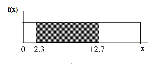
P(c<x<d) is the probability that the random variable X is in the interval between the values c and d. P(c<x<d) is the area under the curve, above the x-axis, to the right of c and the left of d.
P(x=c)=0 The probability that x takes on any single individual value is 0. The area below the curve, above the x-axis, and between x=c and x=c has no width, and therefore no area (area = 0). Since the probability is equal to the area, the probability is also 0.
We will find the area that represents probability by using geometry, formulas, technology, or probability tables. In general, calculus is needed to find the area under the curve for many probability density functions. When we use formulas to find the area in this textbook, the formulas were found by using the techniques of integral calculus. However, because most students taking this course have not studied calculus, we will not be using calculus in this textbook.
There are many continuous probability distributions. When using a continuous probability distribution to model probability, the distribution used is selected to best model and fit the particular situation.
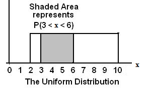
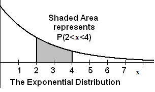
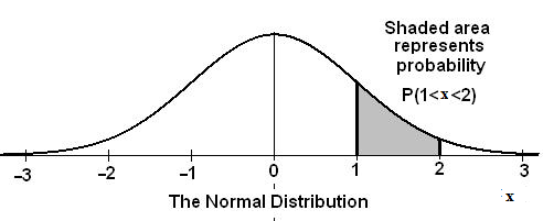
In this chapter and the next chapter, we will study the uniform distribution, the exponential distribution, and the normal distribution. The following graphs illustrate these distributions.
**With contributions from Roberta Bloom
This module introduces the continuous probability function and explores the relationship between the probability of X and the area under the curve of f(X).
We begin by defining a continuous probability density function. We use the function notation f(x). Intermediate algebra may have been your first formal introduction to functions. In the study of probability, the functions we study are special. We define the function f(x) so that the area between it and the x-axis is equal to a probability. Since the maximum probability is one, the maximum area is also one.
For continuous probability distributions, PROBABILITY = AREA.
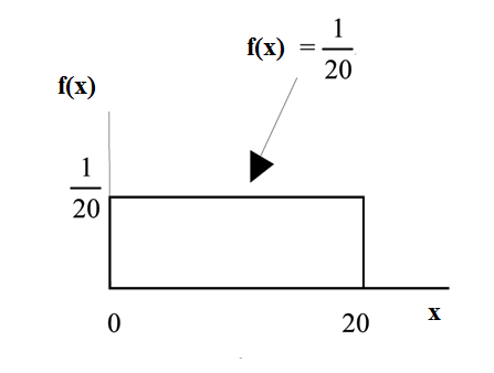
Consider the function
 for
0≤x≤20.
x = a real number.
The graph of
for
0≤x≤20.
x = a real number.
The graph of
 is a horizontal line. However, since
0≤x≤20
,
f(x) is restricted to
the portion between x=0 and
x=20, inclusive .
is a horizontal line. However, since
0≤x≤20
,
f(x) is restricted to
the portion between x=0 and
x=20, inclusive .
 for
0≤x≤20.
for
0≤x≤20.
The graph of  is
a horizontal line segment
when
0≤x≤20.
is
a horizontal line segment
when
0≤x≤20.
The area between  where
0≤x≤20
and the x-axis is the area of a rectangle
with base = 20 and height =
where
0≤x≤20
and the x-axis is the area of a rectangle
with base = 20 and height = .
.

This particular function, where we have restricted x so that the area between the function and the x-axis is 1, is an example of a continuous probability density function. It is used as a tool to calculate probabilities.
Suppose we want to find the area between  and the x-axis where 0<x<2
.
and the x-axis where 0<x<2
.
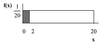

(2–0)=2= base of a rectangle
 = the height.
The area corresponds to a probability. The probability that x is between 0 and 2 is 0.1, which can be written mathematically as P(0<x<2) =P(x<2)=0.1.
Suppose we want to find the area between  and the x-axis where 4<x<15
.
and the x-axis where 4<x<15
.
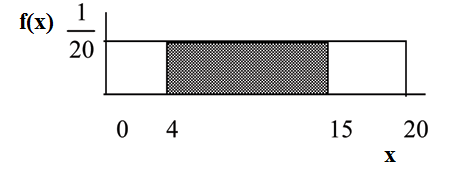

(15–4) = 11 = the base of a rectangle
 = the height.
The area corresponds to the probability P(4<x<15)=0.55.
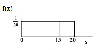
Suppose we want to find P(x = 15). On an x-y graph, x = 15 is a vertical line. A vertical
line has no width (or 0 width). Therefore,  .
.
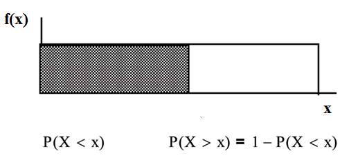
P(X≤x) (can be written as P(X<x) for continuous distributions) is called the cumulative distribution function or CDF. Notice the "less than or equal to" symbol. We can use the CDF to calculate P(X>x) . The CDF gives "area to the left" and P(X>x) gives "area to the right." We calculate P(X>x) for continuous distributions as follows: P(X>x)=1–P(X<x) .
Label the graph with
f(x) and x.
Scale the x and y axes with the maximum x and y values.
 ,
0≤x≤20.
,
0≤x≤20.

Continuous Random Variable: Uniform Distribution is part of the collection col10555 written by Barbara Illowsky and Susan Dean. It describes the properties of the Uniform Distribution with contributions from Roberta Bloom.
The previous problem is an example of the uniform probability distribution.
Illustrate the uniform distribution. The data that follows are 55 smiling times, in seconds, of an eight-week old baby.
| 10.4 | 19.6 | 18.8 | 13.9 | 17.8 | 16.8 | 21.6 | 17.9 | 12.5 | 11.1 | 4.9 |
| 12.8 | 14.8 | 22.8 | 20.0 | 15.9 | 16.3 | 13.4 | 17.1 | 14.5 | 19.0 | 22.8 |
| 1.3 | 0.7 | 8.9 | 11.9 | 10.9 | 7.3 | 5.9 | 3.7 | 17.9 | 19.2 | 9.8 |
| 5.8 | 6.9 | 2.6 | 5.8 | 21.7 | 11.8 | 3.4 | 2.1 | 4.5 | 6.3 | 10.7 |
| 8.9 | 9.4 | 9.4 | 7.6 | 10.0 | 3.3 | 6.7 | 7.8 | 11.6 | 13.8 | 18.6 |
sample mean = 11.49 and sample standard deviation = 6.23
We will assume that the smiling times, in seconds, follow a uniform distribution between 0 and 23 seconds, inclusive. This means that any smiling time from 0 to and including 23 seconds is equally likely. The histogram that could be constructed from the sample is an empirical distribution that closely matches the theoretical uniform distribution.
Let X = length, in seconds, of an eight-week old baby's smile.
The notation for the uniform distribution is
X ~ U(a, b) where a = the lowest value of x and b = the highest value of x.
The probability de