By the end of this chapter, the student should be able to:
Recognize the normal probability distribution and apply it appropriately.
Recognize the standard normal probability distribution and apply it appropriately.
Compare normal probabilities by converting to the standard normal distribution.
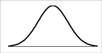
The normal, a continuous distribution, is the most important of all the distributions. It is widely used and even more widely abused. Its graph is bell-shaped. You see the bell curve in almost all disciplines. Some of these include psychology, business, economics, the sciences, nursing, and, of course, mathematics. Some of your instructors may use the normal distribution to help determine your grade. Most IQ scores are normally distributed. Often real estate prices fit a normal distribution. The normal distribution is extremely important but it cannot be applied to everything in the real world.
In this chapter, you will study the normal distribution, the standard normal, and applications associated with them.
Your instructor will record the heights of both men and women in your class, separately. Draw histograms of your data. Then draw a smooth curve through each histogram. Is each curve somewhat bell-shaped? Do you think that if you had recorded 200 data values for men and 200 for women that the curves would look bell-shaped? Calculate the mean for each data set. Write the means on the x-axis of the appropriate graph below the peak. Shade the approximate area that represents the probability that one randomly chosen male is taller than 72 inches. Shade the approximate area that represents the probability that one randomly chosen female is shorter than 60 inches. If the total area under each curve is one, does either probability appear to be more than 0.5?
The normal distribution has two parameters (two numerical descriptive measures), the mean (μ) and the standard deviation (σ). If X is a quantity to be measured that has a normal distribution with mean (μ) and the standard deviation (σ), we designate this by writing
NORMAL:X~N(μ, σ)
The probability density function is a rather complicated function. Do not memorize it. It is not necessary.

The cumulative distribution function is P ( X < x ) . It is calculated either by a calculator or a computer or it is looked up in a table. Technology has made the tables basically obsolete. For that reason, as well as the fact that there are various table formats, we are not including table instructions in this chapter. See the NOTE in this chapter in Calculation of Probabilities.
The curve is symmetrical about a vertical line drawn through the mean, μ. In theory, the mean is the same as the median since the graph is symmetric about μ. As the notation indicates, the normal distribution depends only on the mean and the standard deviation. Since the area under the curve must equal one, a change in the standard deviation, σ, causes a change in the shape of the curve; the curve becomes fatter or skinnier depending on σ. A change in μ causes the graph to shift to the left or right. This means there are an infinite number of normal probability distributions. One of special interest is called the standard normal distribution.
The standard normal distribution is a normal distribution of standardized values called z-scores. A z-score is measured in units of the standard deviation. For example, if the mean of a normal distribution is 5 and the standard deviation is 2, the value 11 is 3 standard deviations above (or to the right of) the mean. The calculation is:
The z-score is 3.
The mean for the standard normal distribution is 0 and the standard deviation is 1. The transformation
 produces the distribution
Z
~
produces the distribution
Z
~
 .
The value x comes from a normal distribution with mean μ and standard deviation σ.
.
The value x comes from a normal distribution with mean μ and standard deviation σ.
If X is a normally distributed random variable and X~N(μ, σ), then the z-score is:
The z-score tells you how many standard deviations that the value x is above (to the right of) or below (to the left of) the mean, μ. Values of x that are larger than the mean have positive z-scores and values of x that are smaller than the mean have negative z-scores. If x equals the mean, then x has a z-score of 0.
Suppose X ~ N(5, 6). This says that X is a normally distributed random variable with mean μ = 5 and standard deviation σ = 6. Suppose x = 17. Then:

This means that x = 17 is 2 standard deviations (2σ) above or to the right of the mean μ = 5. The standard deviation is σ = 6.
Notice that:

Now suppose x=1. Then:

This means that x = 1 is 0.67 standard deviations (- 0.67σ) below or to the left of the mean μ = 5. Notice that:
5
+
(
-0.67
)
(
6
)
is approximately equal to 1
 (This has the pattern
μ
+
(
-0.67
)
σ
=
1
)
(This has the pattern
μ
+
(
-0.67
)
σ
=
1
)
Summarizing, when z is positive, x is above or to the right of μ and when z is negative, x is to the left of or below μ.
Some doctors believe that a person can lose 5 pounds, on the average, in a month by reducing his/her fat intake and by exercising consistently. Suppose weight loss has a normal distribution. Let X = the amount of weight lost (in pounds) by a person in a month. Use a standard deviation of 2 pounds. X~N(5, 2). Fill in the blanks.
Suppose a person lost 10 pounds in a month. The z-score when x = 10 pounds is z = 2.5 (verify). This z-score tells you that x = 10 is ________ standard deviations to the ________ (right or left) of the mean _____ (What is the mean?).
Suppose a person gained 3 pounds (a negative weight loss). Then z = __________. This z-score tells you that x = -3 is ________ standard deviations to the __________ (right or left) of the mean.
Suppose the random variables X and Y have the following normal distributions: X ~ N(5, 6) and Y ~ N(2, 1). If x = 17, then z = 2. (This was previously shown.) If y = 4, what is z?

The z-score for y = 4 is z = 2. This means that 4 is z = 2 standard deviations to the right of the mean. Therefore, x = 17 and y = 4 are both 2 (of their) standard deviations to the right of their respective means.
The z-score allows us to compare data that are scaled differently. To understand the concept, suppose X ~ N(5, 6) represents weight gains for one group of people who are trying to gain weight in a 6 week period and Y ~ N(2, 1) measures the same weight gain for a second group of people. A negative weight gain would be a weight loss. Since x = 17 and y = 4 are each 2 standard deviations to the right of their means, they represent the same weight gain relative to their means.
If X is a random variable and has a normal distribution with mean µ and standard deviation σ then the Empirical Rule says (See the figure below)
About 68.27% of the x values lie between -1σ and +1σ of the mean µ (within 1 standard deviation of the mean).
About 95.45% of the x values lie between -2σ and +2σ of the mean µ (within 2 standard deviations of the mean).
About 99.73% of the x values lie between -3σ and +3σ of the mean µ (within 3 standard deviations of the mean). Notice that almost all the x values lie within 3 standard deviations of the mean.
The z-scores for +1σ and –1σ are +1 and -1, respectively.
The z-scores for +2σ and –2σ are +2 and -2, respectively.
The z-scores for +3σ and –3σ are +3 and -3 respectively.
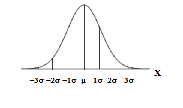
The Empirical Rule is also known as the 68-95-99.7 Rule.
Suppose X has a normal distribution with mean 50 and standard deviation 6.
About 68.27% of the x values lie between -1σ = (-1)(6) = -6 and 1σ = (1)(6) = 6 of the mean 50. The values 50 - 6 = 44 and 50 + 6 = 56 are within 1 standard deviation of the mean 50. The z-scores are -1 and +1 for 44 and 56, respectively.
About 95.45% of the x values lie between -2σ = (-2)(6) = -12 and 2σ = (2)(6) = 12 of the mean 50. The values 50 - 12 = 38 and 50 + 12 = 62 are within 2 standard deviations of the mean 50. The z-scores are -2 and 2 for 38 and 62, respectively.
About 99.73% of the x values lie between -3σ = (-3)(6) = -18 and 3σ = (3)(6) = 18 of the mean 50. The values 50 - 18 = 32 and 50 + 18 = 68 are within 3 standard deviations of the mean 50. The z-scores are -3 and +3 for 32 and 68, respectively.
The arrow in the graph below points to the area to the left of x. This area is represented by the probability P ( X < x ) . Normal tables, computers, and calculators provide or calculate the probability P ( X < x ) .
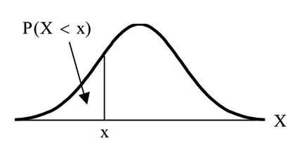
The area to the right is then P ( X > x ) = 1 – P ( X < x ) .
Remember, P ( X < x ) = Area to the left of the vertical line through x.
P ( X > x ) = 1 – P ( X < x ) = . Area to the right of the vertical line through x
P ( X < x ) is the same as P ( X ≤ x ) and P ( X > x ) is the same as P ( X ≥ x ) for continuous distributions.
Probabilities are calculated by using technology. There are instructions in the chapter for the TI-83+ and TI-84 calculators.
In the Table of Contents for Collaborative Statistics, entry 15. Tables has a link to a table of normal probabilities. Use the probability tables if so desired, instead of a calculator. The tables include instructions for how to use then.
If the area to the left is 0.0228, then the area to the right is 1 – 0.0228 = 0.9772 .
The final exam scores in a statistics class were normally distributed with a mean of 63 and a standard deviation of 5.