By the end of this chapter, the student should be able to:
Classify hypothesis tests by type.
Conduct and interpret hypothesis tests for two population means, population standard deviations known.
Conduct and interpret hypothesis tests for two population means, population standard deviations unknown.
Conduct and interpret hypothesis tests for two population proportions.
Conduct and interpret hypothesis tests for matched or paired samples.
Studies often compare two groups. For example, researchers are interested in the effect aspirin has in preventing heart attacks. Over the last few years, newspapers and magazines have reported about various aspirin studies involving two groups. Typically, one group is given aspirin and the other group is given a placebo. Then, the heart attack rate is studied over several years.
There are other situations that deal with the comparison of two groups. For example, studies compare various diet and exercise programs. Politicians compare the proportion of individuals from different income brackets who might vote for them. Students are interested in whether SAT or GRE preparatory courses really help raise their scores.
In the previous chapter, you learned to conduct hypothesis tests on single means and single proportions. You will expand upon that in this chapter. You will compare two means or two proportions to each other. The general procedure is still the same, just expanded.
To compare two means or two proportions, you work with two groups. The groups are classified either as independent or matched pairs. Independent groups mean that the two samples taken are independent, that is, sample values selected from one population are not related in any way to sample values selected from the other population. Matched pairs consist of two samples that are dependent. The parameter tested using matched pairs is the population mean. The parameters tested using independent groups are either population means or population proportions.
This chapter relies on either a calculator or a computer to calculate the degrees of freedom, the test statistics, and p-values. TI-83+ and TI-84 instructions are included as well as the test statistic formulas. When using the TI-83+/TI-84 calculators, we do not need to separate two population means, independent groups, population variances unknown into large and small sample sizes. However, most statistical computer software has the ability to differentiate these tests.
This chapter deals with the following hypothesis tests:
Test of two population means.
Test of two population proportions.
Becomes a test of one population mean.
This module provides an overview of Comparing Two Independent Population Means with Unknown Population Standard Deviations as a part of Collaborative Statistics collection (col10522) by Barbara Illowsky and Susan Dean.
The two independent samples are simple random samples from two distinct populations.
Both populations are normally distributed with the population means and standard deviations unknown unless the sample sizes are greater than 30. In that case, the populations need not be normally distributed.
The test comparing two independent population means with unknown and possibly unequal population standard deviations is called the Aspin-Welch t-test. The degrees of freedom formula was developed by Aspin-Welch.
The comparison of two population means is very common. A difference between
the two samples depends on both the means and the standard deviations. Very
different means can occur by chance if there is great variation among the individual
samples. In order to account for the variation, we take the difference of the sample
means,
 -
-
 , and divide by the standard error (shown below) in order to
standardize the difference. The result is a t-score test statistic (shown below).
, and divide by the standard error (shown below) in order to
standardize the difference. The result is a t-score test statistic (shown below).
Because we do not know the population standard deviations, we estimate them using
the two sample standard deviations from our independent samples. For the
hypothesis test, we calculate the estimated standard deviation, or standard error, of
the difference in sample means,  -
-
 .
.

The test statistic (t-score) is calculated as follows:

s1 and s2, the sample standard deviations, are estimates of σ1 and σ2, respectively.
σ1 and σ2 are the unknown population standard deviations.
 and
and
 are the sample means.
μ1 and μ2 are the population means.
are the sample means.
μ1 and μ2 are the population means.
The degrees of freedom (df) is a somewhat complicated calculation. However, a computer or calculator calculates it easily. The dfs are not always a whole number. The test statistic calculated above is approximated by the student's-t distribution with dfs as follows:

When both sample sizes n1 and n2 are five or larger, the student's-t approximation is very good. Notice that the sample variances s12 and s22 are not pooled. (If the question comes up, do not pool the variances.)
It is not necessary to compute this by hand. A calculator or computer easily computes it.
The average amount of time boys and girls ages 7 through 11 spend playing sports each day is believed to be the same. An experiment is done, data is collected, resulting in the table below. Both populations have a normal distribution.
| Sample Size | Average Number of Hours Playing Sports Per Day | Sample Standard Deviation | |
|---|---|---|---|
| Girls | 9 | 2 hours |  |
| Boys | 16 | 3.2 hours | 1.00 |
Is there a difference in the mean amount of time boys and girls ages 7 through 11 play sports each day? Test at the 5% level of significance.
The population standard deviations are not known. Let g be the subscript for girls and b be the subscript for boys. Then, μg is the population mean for girls and μb is the population mean for boys. This is a test of two independent groups, two population means.
Random variable:
 = difference in the sample mean amount of time girls and boys play sports each day.
Ho:

Ha:

The words "the same" tell you Ho has an "=". Since there are no other words to indicate Ha, then assume "is different." This is a two-tailed test.
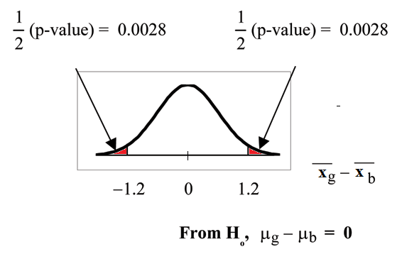
Distribution for the test: Use tdf where df is calculated using the df formula for independent groups, two population means. Using a calculator, df is approximately 18.8462. Do not pool the variances.
Calculate the p-value using a student's-t distribution: p-value = 0.0054
Graph:

sb = 1
So,

Half the p-value is below -1.2 and half is above 1.2.
Make a decision: Since α> p-value, reject Ho.
This means you reject μg = μb. The means are different.
Conclusion: At the 5% level of significance, the sample data show there is sufficient evidence to conclude that the mean number of hours that girls and boys aged 7 through 11 play sports per day is different (mean number of hours boys aged 7 through 11 play sports per day is greater than the mean number of hours played by girls OR the mean number of hours girls aged 7 through 11 play sports per day is greater than the mean number of hours played by boys).
TI-83+ and TI-84: Press STAT. Arrow over to TESTS and press
4:2-SampTTest. Arrow over to Stats and press ENTER. Arrow down
and enter 2 for the first sample mean,
for Sx1, 
9 for n1, 3.2 for the
second sample mean, 1 for Sx2, and 16 for n2. Arrow down to μ1: and
arrow to does not equal μ2. Press ENTER. Arrow down to Pooled: and
No. Press ENTER. Arrow down to Calculate and press ENTER. The
p-value is p = 0.0054, the dfs are approximately 18.8462, and the test
statistic is -3.14. Do the procedure again but instead of Calculate do Draw.
A study is done by a community group in two neighboring colleges to determine which one graduates students with more math classes. College A samples 11 graduates. Their average is 4 math classes with a standard deviation of 1.5 math classes. College B samples 9 graduates. Their average is 3.5 math classes with a standard deviation of 1 math class. The community group believes that a student who graduates from college A has taken more math classes, on the average. Both populations have a normal distribution. Test at a 1% significance level. Answer the following questions.
Is this a test of two means or two proportions?
Are the populations standard deviations known or unknown?
Which distribution do you use to perform the test?
What is the random variable?
What are the null and alternate hypothesis?
Ho : μA ≤ μB
Ha : μA > μB
Is this test right, left, or two tailed?
What is the p-value?
Do you reject or not reject the null hypothesis?
At the 1% level of significance, from the sample data, there is not sufficient evidence to conclude that a student who graduates from college A has taken more math classes, on the average, than a student who graduates from college B.
This module provides an overview of hypothesis testing in situations where there are both two independent population means and known population standard deviations in statistics.
Even though this situation is not likely (knowing the population standard deviations is not likely), the following example illustrates
