This module provides an introduction to Chi-Square Distribution as a part of Collaborative Statistics collection (col10522) by Barbara Illowsky and Susan Dean.
By the end of this chapter, the student should be able to:
Interpret the chi-square probability distribution as the sample size changes.
Conduct and interpret chi-square goodness-of-fit hypothesis tests.
Conduct and interpret chi-square test of independence hypothesis tests.
Conduct and interpret chi-square homogeneity hypothesis tests.
Conduct and interpret chi-square single variance hypothesis tests.
Have you ever wondered if lottery numbers were evenly distributed or if some numbers occurred with a greater frequency? How about if the types of movies people preferred were different across different age groups? What about if a coffee machine was dispensing approximately the same amount of coffee each time? You could answer these questions by conducting a hypothesis test.
You will now study a new distribution, one that is used to determine the answers to the above examples. This distribution is called the Chi-square distribution.
In this chapter, you will learn the three major applications of the Chi-square distribution:
The goodness-of-fit test, which determines if data fit a particular distribution, such as with the lottery example
The test of independence, which determines if events are independent, such as with the movie example
The test of a single variance, which tests variability, such as with the coffee example
Though the Chi-square calculations depend on calculators or computers for most of the calculations, there is a table available (see the Table of Contents 15. Tables). TI-83+ and TI-84 calculator instructions are included in the text.
Look in the sports section of a newspaper or on the Internet for some sports data (baseball averages, basketball scores, golf tournament scores, football odds, swimming times, etc.). Plot a histogram and a boxplot using your data. See if you can determine a probability distribution that your data fits. Have a discussion with the class about your choice.
This module provides an overview of Chi-Square Distribution Notation as a part of Collaborative Statistics collection (col10522) by Barbara Illowsky and Susan Dean.
The notation for the chi-square distribution is:
χ2 ~ χ2df
where df = degrees of freedom depend on how chi-square is being used. (If you want to practice calculating chi-square probabilities then use df = n – 1 . The degrees of freedom for the three major uses are each calculated differently.)
For the
χ2 distribution, the population mean is
μ
=
df
and the population
standard deviation is
 .
.
The random variable is shown as χ2 but may be any upper case letter.
The random variable for a chi-square distribution with k degrees of freedom is the sum of k independent, squared standard normal variables.

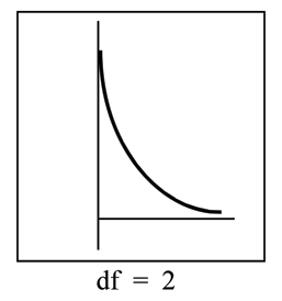
The curve is nonsymmetrical and skewed to the right.
There is a different chi-square curve for each df.
 (a) | 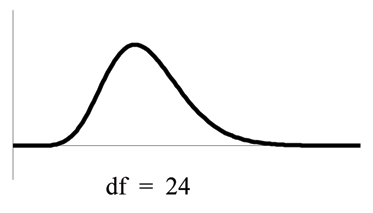 (b) |
The test statistic for any test is always greater than or equal to zero.
When
df
>
90
, the chi-square curve approximates the normal. For
X ~
χ10002
the mean,
μ
=
df
=
1000
and the standard deviation,
 .
Therefore,
X ~
N
(
1000
,
44.7
)
, approximately.
.
Therefore,
X ~
N
(
1000
,
44.7
)
, approximately.
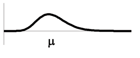
The mean, μ , is located just to the right of the peak.
In the next sections, you will learn about four different applications of the Chi-Square Distribution. These hypothesis tests are almost always right-tailed tests. In order to understand why the tests are mostly right-tailed, you will need to look carefully at the actual definition of the test statistic. Think about the following while you study the next four sections. If the expected and observed values are "far" apart, then the test statistic will be "large" and we will reject in the right tail. The only way to obtain a test statistic very close to zero, would be if the observed and expected values are very, very close to each other. A left-tailed test could be used to determine if the fit were "too good." A "too good" fit might occur if data had been manipulated or invented. Think about the implications of right-tailed versus left-tailed hypothesis tests as you learn the applications of the Chi-Square Distribution.
This module describes how the chi-square distribution is used to conduct goodness-of-fit test.
In this type of hypothesis test, you determine whether the data "fit" a particular distribution or not. For example, you may suspect your unknown data fit a binomial distribution. You use a chi-square test (meaning the distribution for the hypothesis test is chi-square) to determine if there is a fit or not. The null and the alternate hypotheses for this test may be written in sentences or may be stated as equations or inequalities.
The test statistic for a goodness-of-fit test is:

where:
O = observed values (data)
E = expected values (from theory)
k = the number of different data cells or categories
The observed values are the data values and the expected values are the
values you would expect to get if the null hypothesis were true. There are n terms of the form
.
The degrees of freedom are df = (number of categories - 1).
The goodness-of-fit test is almost always right tailed. If the observed values and the corresponding expected values are not close to each other, then the test statistic can get very large and will be way out in the right tail of the chi-square curve.
The expected value for each cell needs to be at least 5 in order to use this test.
Absenteeism of college students from math classes is a major concern to math instructors because missing class appears to increase the drop rate. Suppose that a study was done to determine if the actual student absenteeism follows faculty perception. The faculty expected that a group of 100 students would miss class according to the following chart.
| Number absences per term | Expected number of students |
| 0 - 2 | 50 |
| 3 - 5 | 30 |
| 6 - 8 | 12 |
| 9 - 11 | 6 |
| 12+ | 2 |
A random survey across all mathematics courses was then done to determine the actual number (observed) of absences in a course. The next chart displays the result of that survey.
| Number absences per term | Actual number of students |
| 0 - 2 | 35 |
| 3 - 5 | 40 |
| 6 - 8 | 20 |
| 9 - 11 | 1 |
| 12+ | 4 |
Determine the null and alternate hypotheses needed to conduct a goodness-of-fit test.
Ho: Student absenteeism fits faculty perception.
The alternate hypothesis is the opposite of the null hypothesis.
Ha: Student absenteeism does not fit faculty perception.
Can you use the information as it appears in the charts to conduct the goodness-of-fit test?
| Number absences per term | Expected number of students |
| 0 - 2 | 50 |
| 3 - 5 | 30 |
| 6 - 8 | 12 |
| 9+ | 8 |
| Number absences per term | Actual number of students |
| 0 - 2 | 35 |
| 3 - 5 | 40 |
| 6 - 8 | 20 |
| 9+ | 5 |
What are the degrees of freedom (df)?
There are 4 "cells" or categories in each of the new tables.
df = number of cells - 1 = 4 - 1 = 3
Employers particularly want to know which days of the week employees are absent in a five day work week. Most employers would like to believe that employees are absent equally during the week. Suppose a random sample of 60 managers were asked on which day of the week did they have the highest number of employee absences. The results were distributed as follows:
| Monday | Tuesday | Wednesday | Thursday | Friday | |
|---|---|---|---|---|---|
| Number of Absences | 15 | 12 | 9 | 9 | 15 |
For the population of employees, do the days for the highest number of absences occur with equal frequencies during a five day work week? Test at a 5% significance level.
The null and alternate hypotheses are:
Ho: The absent days occur with equal frequencies, that is, they fit a uniform distribution.
Ha: The absent days occur with unequal frequencies, that is, they do not fit a uniform distribution.
If the absent days occur with equal frequencies, then, out of 60 absent days (the total in the sample: 15 + 12 + 9 + 9 + 15 = 60), there would be 12 absences on Monday, 12 on Tuesday, 12 on Wednesday, 12 on Thursday, and 12 on Friday. These numbers are the expected (E) values. The values in the table are the observed (O) values or data.
This time, calculate the χ2 test statistic by hand. Make a chart with the following headings and fill in the columns:
Expected (E) values (12, 12, 12, 12, 12)
Observed (O) values (15, 12, 9, 9, 15)