This module provides a brief introduction on handling hypothesis tests with two means by the one-way Analysis of Variance (One-Way ANOVA), F Distribution, and the Test of Two Variances statistical analysis.
By the end of this chapter, the student should be able to:
Interpret the F probability distribution as the number of groups and the sample size change.
Discuss two uses for the F distribution: One-Way ANOVA and the test of two variances.
Conduct and interpret One-Way ANOVA.
Conduct and interpret hypothesis tests of two variances.
Many statistical applications in psychology, social science, business administration, and the natural sciences involve several groups. For example, an environmentalist is interested in knowing if the average amount of pollution varies in several bodies of water. A sociologist is interested in knowing if the amount of income a person earns varies according to his or her upbringing. A consumer looking for a new car might compare the average gas mileage of several models.
For hypothesis tests involving more than two averages, statisticians have developed a method called Analysis of Variance" (abbreviated ANOVA). In this chapter, you will study the simplest form of ANOVA called single factor or One-Way ANOVA. You will also study the F distribution, used for One-Way ANOVA, and the test of two variances. This is just a very brief overview of One-Way ANOVA. You will study this topic in much greater detail in future statistics courses.
One-Way ANOVA, as it is presented here, relies heavily on a calculator or computer.
For further information about One-Way ANOVA, use the online link ANOVA. Use the back button to return here. (The url is http://en.wikipedia.org/wiki/Analysis_of_variance.)
This module describes the assumptions needed for implementing an One-Way ANOVA and how to set up the hypothesis test for the ANOVA.
The purpose of a One-Way ANOVA test is to determine the existence of a statistically significant difference among several group means. The test actually uses variances to help determine if the means are equal or not.
In order to perform a One-Way ANOVA test, there are five basic assumptions to be fulfilled:
Each population from which a sample is taken is assumed to be normal.
Each sample is randomly selected and independent.
The populations are assumed to have equal standard deviations (or variances).
The factor is the categorical variable.
The response is the numerical variable.
The null hypothesis is simply that all the group population means are the same. The alternate hypothesis is that at least one pair of means is different. For example, if there are k groups:
Ho : μ1 = μ2 = μ3 = ... = μk
Ha : At least two of the group means μ1 , μ2 , μ3 , ... , μk are not equal.
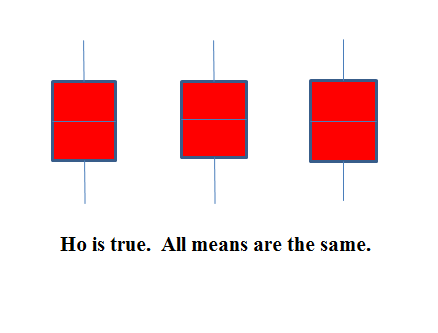
The graphs help in the understanding of the hypothesis test. In the first graph (red box plots),
Ho
:
μ1
=
μ2
=
μ3
and the three populations have the same distribution if the null hypothesis is true. The variance of the combined data is approximately the same as the variance of each of the populations.
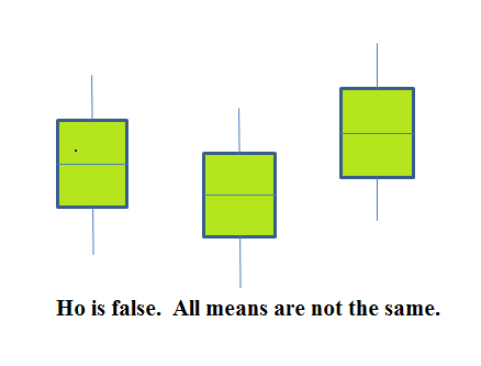
If the null hypothesis is false, then the variance of the combined data is larger which is caused by the different means as shown in the second graph (green box plots).
This module describes how to calculate the F Ratio and F Distribution based on the hypothesis test for the One-Way ANOVA.
The distribution used for the hypothesis test is a new one. It is called the F distribution, named after Sir Ronald Fisher, an English statistician. The F statistic is a ratio (a fraction). There are two sets of degrees of freedom; one for the numerator and one for the denominator.
For example, if F follows an F distribution and the degrees of freedom for the numerator are 4 and the degrees of freedom for the denominator are 10, then F ~ F 4 , 10 .
The F distribution is derived from the Student's-t distribution. One-Way ANOVA expands the t-test for comparing more than two groups. The scope of that derivation is beyond the level of this course.
To calculate the F ratio, two estimates of the variance are made.
Variance between samples: An estimate of σ2 that is the variance of the sample means multiplied by n (when there is equal n). If the samples are different sizes, the variance between samples is weighted to account for the different sample sizes. The variance is also called variation due to treatment or explained variation.
Variance within samples: An estimate of σ2 that is the average of the sample variances (also known as a pooled variance). When the sample sizes are different, the variance within samples is weighted. The variance is also called the variation due to error or unexplained variation.
SSbetween = the sum of squares that represents the variation among the different samples.
SSwithin = the sum of squares that represents the variation within samples that is due to chance.
To find a "sum of squares" means to add together squared quantities which, in some cases, may be weighted. We used sum of squares to calculate the sample variance and the sample standard deviation in Descriptive Statistics.
MS means "mean square." MSbetween is the variance between groups and MSwithin is the variance within groups.
k = the number of different groups
nj = the size of the
 group
group
sj= the sum of the values in the
 group
group
n = total number of all the values combined. (total sample size: ∑nj)
x = one value: ∑x=∑sj
Sum of squares of all values from every group combined: ∑x2
Between group variability: 
Total sum of squares:

Explained variation- sum of squares representing variation among the different samples

Unexplained variation- sum of squares representing variation within samples due to chance:

df's for different groups (df's for the numerator):

Equation for errors within samples (df's for the denominator):

Mean square (variance estimate) explained by the different groups:

Mean square (variance estimate) that is due to chance (unexplained): 
MSbetween and MSwithin can be written as follows:


The One-Way ANOVA test depends on the fact that MSbetween can be influenced by population differences among means of the several groups. Since MSwithin compares values of each group to its own group mean, the fact that group means might be different does not affect MSwithin.
The null hypothesis says that all groups are samples from populations having the same normal distribution. The alternate hypothesis says that at least two of the sample groups come from populations with different normal distributions. If the null hypothesis is true, MSbetween and MSwithin should both estimate the same value.
The null hypothesis says that all the group population means are equal. The hypothesis of equal means implies that the populations have the same normal distribution because it is assumed that the populations are normal and that they have equal variances.

If MSbetween and MSwithin estimate the same value (following the belief that Ho is true), then the F-ratio should be approximately equal to 1. Mostly just sampling errors would contribute to variations away from 1. As it turns out, MSbetween consists of the population variance plus a variance produced from the differences between the samples. MSwithin is an estimate of the population variance. Since variances are always positive, if the null hypothesis is false, MSbetween will generally be larger than MSwithin. Then the F-ratio will be larger than 1. However, if the population effect size is small it is not unlikely that MSwithin will be larger in a give sample.
The above calculations were done with groups of different sizes. If the groups are the same size, the calculations simplify somewhat and the F ratio can be written as:

n=the sample size


s2pooled= the mean of the sample variances (pooled variance)
 the variance of the sample means
The data is typically put into a table for easy viewing. One-Way ANOVA results are often displayed in this manner by computer software.
| Source of Variation | Sum of Squares (SS) | Degrees of Freedom (df) | Mean Square (MS) | F |
|---|---|---|---|---|
| Factor (Between) | SS(Factor) | k - 1 | MS(Factor) = SS(Factor)/(k-1) | F = MS(Factor)/MS(Error) |
| Error (Within) | SS(Error) | n - k | MS(Error) = SS(Error)/(n-k) | |
| Total | SS(Total) | n - 1 |
Three different diet plans are to be tested for mean weight loss. The entries in the table are the weight losses for the different plans. The One-Way ANOVA table is shown below.
| Plan 1 | Plan 2 | Plan 3 |
|---|---|---|
| 5 | 3.5 | 8 |
| 4.5 | 7 | 4 |
| 4 | 3.5 | |
| 3 | 4.5 |
One-Way ANOVA Table: The formulas for SS(Total), SS(Factor) = SS(Between) and SS(Error) = SS(Within) are shown above. This same information is provided by the TI calculator hypothesis test function ANOVA in STAT TESTS (syntax is ANOVA(L1, L2, L3) where L1, L2, L3 have the data from Plan 1, Plan 2, Plan 3 respectively).
| Source of Variation | Sum of Squares (SS) | Degrees of Freedom (df) | Mean Square (MS) | F |
|---|---|---|---|---|
| Factor (Between) | SS(Factor) = SS(Between) =2.2458 | k - 1 = 3 groups - 1 = 2 | MS(Factor) = SS(Factor)/(k-1) = 2.2458/2 = 1.1229 | F = MS(Factor)/MS(Error) = 1.1229/2.9792 = 0.3769 |
| Error (Within) | SS(Error) = SS(Within) = 20.8542 | n - k = 10 total data - 3 groups = 7 | MS(Error) = SS(Error)/(n-k) = 20.8542/7 = 2.9792 | |
| Total | SS(Total)
|