This module provides an introduction of Linear Regression and Correlation as a part of Collaborative Statistics collection (col10522) by Barbara Illowsky and Susan Dean.
By the end of this chapter, the student should be able to:
Discuss basic ideas of linear regression and correlation.
Create and interpret a line of best fit.
Calculate and interpret the correlation coefficient.
Calculate and interpret outliers.
Professionals often want to know how two or more numeric variables are related. For example, is there a relationship between the grade on the second math exam a student takes and the grade on the final exam? If there is a relationship, what is it and how strong is the relationship?
In another example, your income may be determined by your education, your profession, your years of experience, and your ability. The amount you pay a repair person for labor is often determined by an initial amount plus an hourly fee. These are all examples in which regression can be used.
The type of data described in the examples is bivariate data - "bi" for two variables. In reality, statisticians use multivariate data, meaning many variables.
In this chapter, you will be studying the simplest form of regression, "linear regression" with one independent variable (x). This involves data that fits a line in two dimensions. You will also study correlation which measures how strong the relationship is.
This module provides an overview of Linear Regression and Correlation: Linear Equations as a part of Collaborative Statistics collection (col10522) by Barbara Illowsky and Susan Dean.
Linear regression for two variables is based on a linear equation with one independent variable. It has the form:
where a and b are constant numbers.
x is the independent variable, and y is the dependent variable. Typically, you choose a value to substitute for the independent variable and then solve for the dependent variable.
The following examples are linear equations.
The graph of a linear equation of the form y = a + bx is a straight line. Any line that is not vertical can be described by this equation.
Linear equations of this form occur in applications of life sciences, social sciences, psychology, business, economics, physical sciences, mathematics, and other areas.
Aaron's Word Processing Service (AWPS) does word processing. Its rate is $32 per hour plus a $31.50 one-time charge. The total cost to a customer depends on the number of hours it takes to do the word processing job.
Find the equation that expresses the total cost in terms of the number of hours required to finish the word processing job.
Let x = the number of hours it takes to get the job done.
Let y = the total cost to the customer.
The $31.50 is a fixed cost. If it takes x hours to complete the job, then (32)(x) is the cost of the word processing only. The total cost is:
y=31.50+32x
This module provides an overview of Linear Regression and Correlation: Slope and Y-Intercept of a Linear Equation as a part of Collaborative Statistics collection (col10522) by Barbara Illowsky and Susan Dean.
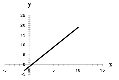
For the linear equation y = a + bx , b = slope and a = y-intercept.
From algebra recall that the slope is a number that describes the steepness of a line and the y-intercept is the y coordinate of the point (0,a) where the line crosses the y-axis.
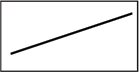 (a)
If b>0, the line slopes upward to the right.
| 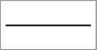 (b)
If b=0, the line is horizontal.
| 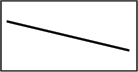 (c)
If b<0, the line slopes downward to the right.
|
Svetlana tutors to make extra money for college. For each tutoring session, she charges a one time fee of $25 plus $15 per hour of tutoring. A linear equation that expresses the total amount of money Svetlana earns for each session she tutors is y=25+15x.
What are the independent and dependent variables? What is the y-intercept and what is the slope? Interpret them using complete sentences.
The independent variable (x) is the number of hours Svetlana tutors each session. The dependent variable (y) is the amount, in dollars, Svetlana earns for each session.
The y-intercept is 25 (a = 25). At the start of the tutoring session, Svetlana charges a one-time fee of $25 (this is when x = 0). The slope is 15 (b = 15). For each session, Svetlana earns $15 for each hour she tutors.
This module provides an overview of Linear Regression and Correlation: Scatter Plots as a part of Collaborative Statistics collection (col10522) by Barbara Illowsky and Susan Dean.
Before we take up the discussion of linear regression and correlation, we need to examine a way to display the relation between two variables x and y. The most common and easiest way is a scatter plot. The following example illustrates a scatter plot.
From an article in the Wall Street Journal: In Europe and Asia, m-commerce is popular. M-commerce users have special mobile phones that work like electronic wallets as well as provide phone and Internet services. Users can do everything from paying for parking to buying a TV set or soda from a machine to banking to checking sports scores on the Internet. For the years 2000 through 2004, was there a relationship between the year and the number of m-commerce users? Construct a scatter plot. Let x = the year and let y = the number of m-commerce users, in millions.
(a) Table showing the number of m-commerce users (in millions) by year. | 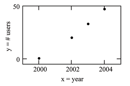 (b)
Scatter plot showing the number of m-commerce users (in millions) by year. |
A scatter plot shows the direction and strength of a relationship between the variables. A clear direction happens when there is either:
High values of one variable occurring with high values of the other variable or low values of one variable occurring with low values of the other variable.
High values of one variable occurring with low values of the other variable.
You can determine the strength of the relationship by looking at the scatter plot and seeing how close the points are to a line, a power function, an exponential function, or to some other type of function.
When you look at a scatterplot, you want to notice the overall pattern and any deviations from the pattern. The following scatterplot examples illustrate these concepts.
<db:title> Positive Linear Pattern (Strong)</db:title> 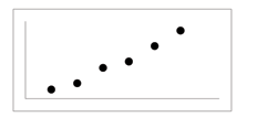 (a) | <db:title> Linear Pattern w/ One Deviation</db:title> 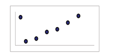 (b) |
<db:title> Negative Linear Pattern (Strong)</db:title> 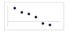 (a) | <db:title> Negative Linear Pattern (Weak)</db:title> 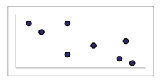 (b) |
<db:title> Exponential Growth Pattern</db:title> 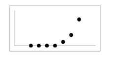 (a) | <db:title> No Pattern</db:title> 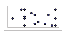 (b) |
In this chapter, we are interested in scatter plots that show a linear pattern. Linear patterns are quite common. The linear relationship is strong if the points are close to a straight line. If we think that the points show a linear relationship, we would like to draw a line on the scatter plot. This line can be calculated through a process called linear regression. However, we only calculate a regression line if one of the variables helps to explain or predict the other variable. If x is the independent variable and y the dependent variable, then we can use a regression line to predict y for a given value of x.
Linear Regression and Correlation: The Regression Equation is a part of Collaborative Statistics collection (col10522) by Barbara Illowsky and Susan Dean. Contributions from Roberta Bloom include instructions for finding and graphing the regression equation and scatterplot using the LinRegTTest on the TI-83,83+,84+ calculators.
Data rarely fit a straight line exactly. Usually, you must be satisfied with rough predictions. Typically, you have a set of data whose scatter plot appears to "fit" a straight line. This is called a Line of Best Fit or Least Squares Line.
If you know a person's pinky (smallest) finger length, do you think you could predict that person's height? Collect data from your class (pinky finger length, in inches). The independent variable, x, is pinky finger length and the dependent variable, y, is height.
For each set of data, plot the points on graph paper. Make your graph big enough and use a ruler. Then "by eye" draw a line that appears to "fit" the data. For your line, pick two convenient points and use them to find the slope of the line. Find the y-intercept of the line by extending your lines so they cross the y-axis. Using the slopes and the y-intercepts, write your equation of "best fit". Do you think everyone will have the same equation? Why or why not?
Using your equation, what is the predicted height for a pinky length of 2.5 inches?
A random sample of 11 statistics students produced the following data where x is the third exam score, out of 80, and y is the final exam score, out of 200. Can you predict the final exam score of a random student if you know the third exam score?
|