Digital transformation of the sampling rate of signals, or signal processing with different sampling rates in the system.
Sampling-rate conversion: CD to DAT format change, for example.
Improved D/A, A/D conversion: oversampling converters; which reduce performance requirements on anti-aliasing or reconstruction filters
FDM channel modulation and processing: bandwidth of individual channels is much less than the overall bandwidth
Subband coding of speech and images: Eyes and ears are not as sensitive to errors in higher frequency bands, so many coding schemes split signals into different frequency bands and quantize higher-frequency bands with much less precision.
This procedure is motivated by an analog-based method: one conceptually simple method to change the sampling rate is to simply convert a digital signal to an analog signal and resample it! (Figure 6.1)

 Recall the ideal D/A:

The problems with this scheme are:
A/D, D/A, filters cost money
imperfections in these devices introduce errors
Digital implementation of rate-changing according to this formula has three problems:
Infinite sum: The solution is to truncate. Consider
sinct≈0
for
t<t1,
t>t2: Then
mT1−nT0<t1 and
mT1−nT0>t2 which implies


This is essentially lowpass filter design using a boxcar window: other finite-length filter design methods could be used for this.
Lack of causality: The solution is to delay by max{|N|} samples. The mathematics of the analog portions of this system can be implemented digitally.


So we have an all-digital formula for exact digital-to-digital rate changing!
Cost of computing
sincT′(mT1−nT0)
: The solution is to precompute the table of
sinc(t)
values. However, if
 is not a rational fraction, an infinite number of
samples will be needed, so some approximation will have to
be tolerated.
is not a rational fraction, an infinite number of
samples will be needed, so some approximation will have to
be tolerated.
Rate transformation of any rate to any other rate can be accomplished digitally with arbitrary precision (if some delay is acceptable). This method is used in practice in many cases. We will examine a number of special cases and computational improvements, but in some sense everything that follows are details; the above idea is the central idea in multirate signal processing.
Useful references for the traditional material (everything except PRFBs) are Crochiere and Rabiner, 1981 [link] and Crochiere and Rabiner, 1983 [link]. A more recent tutorial is Vaidyanathan [link]; see also Rioul and Vetterli [link]. References to most of the original papers can be found in these tutorials.
R.E. Crochiere and L.R. Rabiner. (1981, March). Interpolation and Decimation of Digital Signals: A Tutorial Review. Proc. IEEE, 69(3), 300-331.
R.E. Crochiere and L.R. Rabiner. (1983). Multirate Digital Signal Processing. Englewood Cliffs, NJ: Prentice-Hall.
P.P Vaidyanathan. (1990, January). Multirate Digital Filters, Filter Banks, Polyphase Networks, and Applications: A Tutorial. Proc. IEEE, 78(1), 56-93.
O. Rioul and M. Vetterli. (1991, October). Wavelets and Signal Processing. IEEE Signal Processing Magazine, 8(4), 14-38.
Interpolation means increasing the sampling rate, or filling in in-between samples. Equivalent to sampling a bandlimited analog signal L times faster. For the ideal interpolator,
We wish to accomplish this digitally. Consider Equation and Figure 6.2.
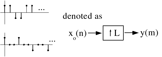
The DTFT of y(m) is

Since
X0(ω′)
is periodic with a period of
2π
,
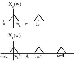
X0(Lω)=Y(ω)
is periodic with a period of
(see Figure 6.3).
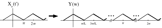
By inserting zero samples between the samples of x0(n) , we obtain a signal with a scaled frequency response that simply replicates X0(ω′) L times over a 2π interval!
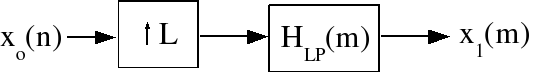
Obviously, the desired x1(m) can be obtained simply by lowpass filtering y(m) to remove the replicas.
Given
In practice, a finite-length lowpass filter is designed using
any of the methods studied so far (Figure 6.4).
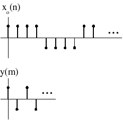
Let y(m)=x0(Lm) (Figure 6.5)
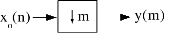
That is, keep only every Lth sample (Figure 6.6)
In frequency (DTFT):

Now
 for
|ω|<π
as shown in homework #1 , where
X(k)
is the DFT of one period of the periodic sequence.
In this case,
X(k)=1
for
k∈{0, 1, …, M−1}
and
for
|ω|<π
as shown in homework #1 , where
X(k)
is the DFT of one period of the periodic sequence.
In this case,
X(k)=1
for
k∈{0, 1, …, M−1}
and
 .
.

so
 i.e., we get digital
aliasing.(Figure 6.7)
i.e., we get digital
aliasing.(Figure 6.7)
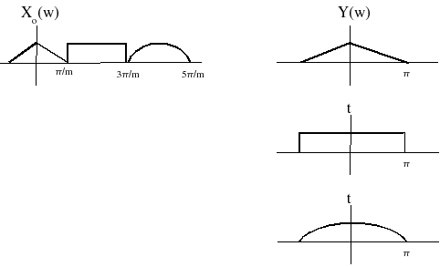
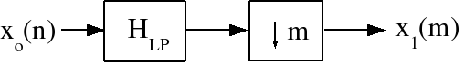
Usually, we prefer not to have aliasing, so the downsampler
is preceded by a lowpass filter to remove all frequency
components above
 (Figure 6.8).
This is easily accomplished by interpolating by a factor of L, then decimating by a factor of M (Figure 6.9).

The two lowpass filters can be combined into one LP filter
with the lower cutoff,
 Obviously, the computational complexity and simplicity of
implementation will depend on
Obviously, the computational complexity and simplicity of
implementation will depend on
 :
2/3
will be easier to implement than
1061/1060
!
:
2/3
will be easier to implement than
1061/1060
!
Rate-changing appears expensive computationally, since for both decimation and interpolation the lowpass filter is implemented at the higher rate. However, this is not necessary.
For the interpolator, most of the samples in the upsampled signal are zero, and thus require no computation. (Figure 6.10)
For
and
p=mmodL
,
gp(n)=h(Ln+p) Pictorially, this can be represented as in Figure 6.11.
These are called polyphase structures, and the gp(n) are called polyphase filters.
If h(m) is a length-N filter:
No simplification:

Polyphase structure:
where L is the number of filters,
is the taps/filter, and
 is the rate.
Thus we save a factor of L by not being dumb.
For a given precision, N is proportional to L, (why?), so the computational cost does increase with the interpolation rate.