In many applications requiring filtering, the necessary frequency response may not be known beforehand, or it may vary with time. (Example; suppression of engine harmonics in a car stereo.) In such applications, an adaptive filter which can automatically design itself and which can track system variations in time is extremely useful. Adaptive filters are used extensively in a wide variety of applications, particularly in telecommunications.
Wiener Filters: L2 optimal (FIR) filter design in a statistical context
LMS algorithm: simplest and by-far-the-most-commonly-used adaptive filter algorithm
Stability and performance of the LMS algorithm: When and how well it works
Applications of adaptive filters: Overview of important applications
Introduction to advanced adaptive filter algorithms: Techniques for special situations or faster convergence
Stochastic L2 optimal (least squares) FIR filter design problem: Given a wide-sense stationary (WSS) input signal xk and desired signal dk (WSS ⇔ E[yk]=E[yk+d] , ryz(l)=E[ykzk+l] , ryy(0)<∞ )
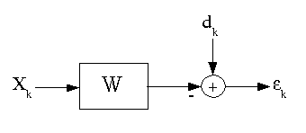
The Wiener filter is the linear, time-invariant filter minimizing E[ε2] , the variance of the error.
As posed, this problem seems slightly silly, since dk is already available! However, this idea is useful in a wide cariety of applications.
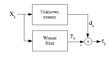
System identification (radar, non-destructive testing, adaptive control systems)
Usually one desires that the input signal xk be "persistently exciting," which, among other things, implies non-zero energy in all frequency bands. Why is this desirable?
for convenience, we will analyze only the causal, real-data case; extensions are straightforward.


 where
rdd(0)=E[dk2]
rdx(l)=E[dkXk
–
l
]
rxx(l−m)=E[xkxk
+
l
–
m
]
This can be written in matrix form as
E[ε2]=rdd(0)−2PWT+WTRW
where
where
rdd(0)=E[dk2]
rdx(l)=E[dkXk
–
l
]
rxx(l−m)=E[xkxk
+
l
–
m
]
This can be written in matrix form as
E[ε2]=rdd(0)−2PWT+WTRW
where

 To solve for the optimum filter, compute the gradient with
respect to the top weights vector W
To solve for the optimum filter, compute the gradient with
respect to the top weights vector W
 ∇=–(2P)+2RW
(recall
∇=–(2P)+2RW
(recall
 ,
,
 for symmetric M) setting the
gradient equal to zero ⇒
for symmetric M) setting the
gradient equal to zero ⇒
 Since R is a correlation matrix,
it must be non-negative definite, so this is a minimizer. For
R positive definite, the
minimizer is unique.
Since R is a correlation matrix,
it must be non-negative definite, so this is a minimizer. For
R positive definite, the
minimizer is unique.
The weiner-filter,
 , is ideal for many applications. But several issues
must be addressed to use it in practice.
, is ideal for many applications. But several issues
must be addressed to use it in practice.
In practice one usually won't know exactly the statistics of xk and dk (i.e. R and P) needed to compute the Weiner filter.
How do we surmount this problem?

 then solve

How can
 be computed efficiently?
how does one choose N?
Larger N → more
accurate estimates of the correlation values →
better
. However, larger N
leads to slower adaptation.
The success of adaptive systems depends on x, d being roughly stationary over at least N samples, N>M . That is, all adaptive filtering algorithms require that the underlying system varies slowly with respect to the sampling rate and the filter length (although they can tolerate occasional step discontinuities in the underlying system).
As presented here, an adaptive filter requires computing a matrix inverse at each sample. Actually, since the matrix R is Toeplitz, the linear system of equations can be sovled with O(M2) computations using Levinson's algorithm, where M is the filter length. However, in many applications this may be too expensive, especially since computing the filter output itself requires O(M) computations. There are two main approaches to resolving the computation problem
Take advantage of the fact that Rk+1 is only slightly changed from Rk to reduce the computation to O(M) ; these algorithms are called Fast Recursive Least Squareds algorithms; all methods proposed so far have stability problems and are dangerous to use.
Find a different approach to solving the optimization problem that doesn't require explicit inversion of the correlation matrix.
Adaptive algorithms involving the correlation matrix are called Recursive least Squares (RLS) algorithms. Historically, they were developed after the LMS algorithm, which is the slimplest and most widely used approach O(M) . O(M2) RLS algorithms are used in applications requiring very fast adaptation.
The least squares optimal filter design problem is quadratic in the filter coefficients: E[ε2]=rdd(0)−2PTW+WTRW If R is positive definite, the error surface E[ε2](w0, w1, …, wM – 1 ) is a unimodal "bowl" in ℝN.
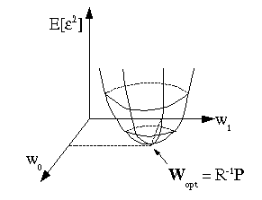
The problem is to find the bottom of the bowl. In an adaptive filter context, the shape and bottom of the bowl may drift slowly with time; hopefully slow enough that the adaptive algorithm can track it.
For a quadratic error surface, the bottom of the bowl can be found in one step by computing R-1P . Most modern nonlinear optimization methods (which are used, for example, to solve the LP optimal IIR filter design problem!) locally approximate a nonlinear function with a second-order (quadratic) Taylor series approximation and step to the bottom of this quadratic approximation on each iteration. However, an older and simpler appraoch to nonlinear optimaztion exists, based on gradient descent.
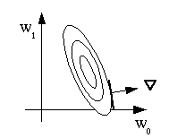
The idea is to iteratively find the minimizer by computing
the gradient of the error function:
. The gradient is a vector in
ℝM pointing in the steepest uphill direction on the
error surface at a given point
Wi, with ∇ having a
magnitude proportional to the slope of the error surface in
this steepest direction.
By updating the coefficient vector by taking a step opposite the gradient direction : Wi+1=Wi−μ∇i, we go (locally) "downhill" in the steepest direction, which seems to be a sensible way to iteratively solve a nonlinear optimization problem. The performance obviously depends on μ; if μ is too large, the iterations could bounce back and forth up out of the bowl. However, if μ is too small, it could take many iterations to approach the bottom. We will determine criteria for choosing μ later.
In summary, the gradient descent algorithm for solving the Weiner filter problem is: Guess W0 do i=1 , ∞ ∇i=–(2P)+2R