Mathematically, analog signals are functions having as their independent variables continuous quantities, such as space and time. Discrete-time signals are functions defined on the integers; they are sequences. As with analog signals, we seek ways of decomposing discrete-time signals into simpler components. Because this approach leading to a better understanding of signal structure, we can exploit that structure to represent information (create ways of representing information with signals) and to extract information (retrieve the information thus represented). For symbolic-valued signals, the approach is different: We develop a common representation of all symbolic-valued signals so that we can embody the information they contain in a unified way. From an information representation perspective, the most important issue becomes, for both real-valued and symbolic-valued signals, efficiency: what is the most parsimonious and compact way to represent information so that it can be extracted later.
A discrete-time signal is represented symbolically as s(n) , where n={…, -1, 0, 1, …} .
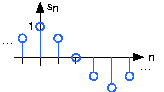
We usually draw discrete-time signals as stem plots to emphasize the fact they are functions defined only on the integers. We can delay a discrete-time signal by an integer just as with analog ones. A signal delayed by m samples has the expression s(n−m) .
The most important signal is, of course, the complex exponential sequence.
Note that the frequency variable f is dimensionless and that adding an integer to the frequency of the discrete-time complex exponential has no effect on the signal's value.

This derivation follows because the complex exponential evaluated at an integer multiple of 2π equals one. Thus, we need only consider frequency to have a value in some unit-length interval.
Discrete-time sinusoids have the obvious form
s(n)=Acos(2πfn+φ)
. As opposed to analog complex exponentials and
sinusoids that can have their frequencies be any real value,
frequencies of their discrete-time counterparts yield unique
waveforms only when
f
lies in the interval
 . This choice of frequency interval is arbitrary; we can also choose the frequency to lie in the interval
[0, 1)
.
How to choose a unit-length interval for a sinusoid's frequency will become evident later.
. This choice of frequency interval is arbitrary; we can also choose the frequency to lie in the interval
[0, 1)
.
How to choose a unit-length interval for a sinusoid's frequency will become evident later.
The second-most important discrete-time signal is the unit sample, which is defined to be

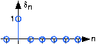
Examination of a discrete-time signal's plot, like that of the cosine signal shown in Figure 1.1, reveals that all signals consist of a sequence of delayed and scaled unit samples. Because the value of a sequence at each integer m is denoted by s(m) and the unit sample delayed to occur at m is written δ(n−m) , we can decompose any signal as a sum of unit samples delayed to the appropriate location and scaled by the signal value.

This kind of decomposition is unique to discrete-time signals, and will prove useful subsequently.
The unit sample in discrete-time is well-defined at the origin, as opposed to the situation with analog signals.

An interesting aspect of discrete-time signals is that their values do not need to be real numbers. We do have real-valued discrete-time signals like the sinusoid, but we also have signals that denote the sequence of characters typed on the keyboard. Such characters certainly aren't real numbers, and as a collection of possible signal values, they have little mathematical structure other than that they are members of a set. More formally, each element of the symbolic-valued signal s(n) takes on one of the values {a1, …, aK} which comprise the alphabet A . This technical terminology does not mean we restrict symbols to being members of the English or Greek alphabet. They could represent keyboard characters, bytes (8-bit quantities), integers that convey daily temperature. Whether controlled by software or not, discrete-time systems are ultimately constructed from digital circuits, which consist entirely of analog circuit elements. Furthermore, the transmission and reception of discrete-time signals, like e-mail, is accomplished with analog signals and systems. Understanding how discrete-time and analog signals and systems intertwine is perhaps the main goal of this course.
Discrete-time systems can act on discrete-time signals in ways similar to those found in analog signals and systems. Because of the role of software in discrete-time systems, many more different systems can be envisioned and "constructed" with programs than can be with analog signals. In fact, a special class of analog signals can be converted into discrete-time signals, processed with software, and converted back into an analog signal, all without the incursion of error. For such signals, systems can be easily produced in software, with equivalent analog realizations difficult, if not impossible, to design.
A discrete-time signal s(n) is delayed by n0 samples when we write s(n−n0) , with n0>0 . Choosing n0 to be negative advances the signal along the integers. As opposed to analog delays, discrete-time delays can only be integer valued. In the frequency domain, delaying a signal corresponds to a linear phase shift of the signal's discrete-time Fourier transform: (s(n−n0) ↔ ⅇ–(ⅈ2πfn0)S(ⅇⅈ2πf)) .
Linear discrete-time systems have the superposition property.
A discrete-time system is called shift-invariant (analogous to time-invariant analog systems) if delaying the input delays the corresponding output.
We use the term shift-invariant to emphasize that delays can only have integer values in discrete-time, while in analog signals, delays can be arbitrarily valued.
We want to concentrate on systems that are both linear and shift-invariant. It will be these that allow us the full power of frequency-domain analysis and implementations. Because we have no physical constraints in "constructing" such systems, we need only a mathematical specification. In analog systems, the differential equation specifies the input-output relationship in the time-domain. The corresponding discrete-time specification is the difference equation.
Here, the output signal y(n) is related to its past values y(n−l) , l={1, …, p} , and to the current and past values of the input signal x(n) . The system's characteristics are determined by the choices for the number of coefficients p and q and the coefficients' values {a1, …, ap} and {b0, b1, …, bq} .
There is an asymmetry in the coefficients: where is a0 ? This coefficient would multiply the y(n) term in the difference equation. We have essentially divided the equation by it, which does not change the input-output relationship. We have thus created the convention that a0 is always one.
As opposed to differential equations, which only provide an implicit description of a system (we must somehow solve the differential equation), difference equations provide an explicit way of computing the output for any input. We simply express the difference equation by a program that calculates each output from the previous output values, and the current and previous inputs.
Convolution, one of the most important concepts in electrical engineering, can be used to determine the output a system produces for a given input signal. It can be shown that a linear time invariant system is completely characterized by its impulse response. The sifting property of the discrete time impulse function tells us that the input signal to a system can be represented as a sum of scaled and shifted unit impulses. Thus, by linearity, it would seem reasonable to compute of the output signal as the sum of scaled and shifted unit impulse responses. That is exactly what the operation of convolution accomplishes. Hence, convolution can be used to determine a linear time invariant system's output from knowledge of the input and the impulse response.
Discrete time convolution is an operation on two discrete time signals defined by the integral

for all signals f,g defined on Z. It is important to note that the operation of convolution is commutative, meaning that
for all signals f,g defined on Z. Thus, the convolution operation could have been just as easily stated using the equivalent definition
for all signals f,g defined on Z. Convolution has several other important properties not listed here but explained and derived in a later module.
The above operation definition has been chosen to be particularly useful in the study of linear time invariant systems. In order to see this, consider a linear time invariant system H with unit impulse response h. Given a system input signal x we would like to compute the system output signal H(x). First, we note that the input can be expressed as the convolution

by the sifting property of the unit impulse function. By linearity

Since Hδ(n–k) is the shifted unit impulse response h(n–k), this gives the result
Hence, convolution has been defined such that the output of a linear time invariant system is given by the convolution of the system input with the system unit impulse response.
It is often helpful to be able to visualize the computation of a convolution in terms of graphical processes. Consider the convolution of two functions f,g given by

The first step in graphically understanding the operation of convolution is to plot each of the functions. Next, one of the functions must be selected, and its plot reflected across the k=0 axis. For each real t, that same function must be shifted left by t. The product of the two resulting plots is then constructed. Finally, the area under the resulting curve is computed.
Recall that the impulse response for a discrete time echoing feedback system with gain a is