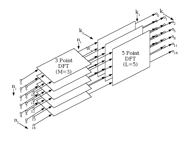
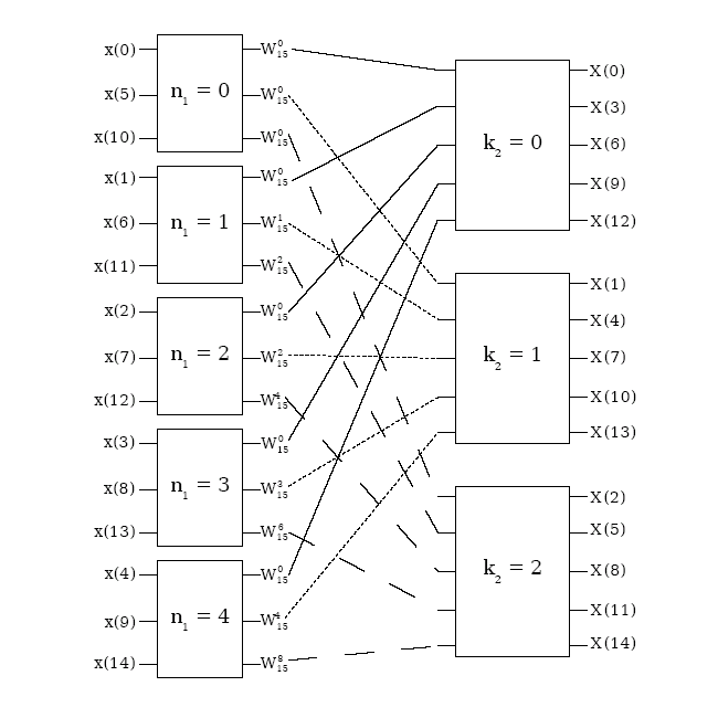
The discrete Fourier transform (DFT) is the primary transform used for numerical computation in digital signal processing. It is very widely used for spectrum analysis, fast convolution, and many other applications. The DFT transforms N discrete-time samples to the same number of discrete frequency samples, and is defined as

The DFT is widely used in part because it can be computed very efficiently using fast Fourier transform (FFT) algorithms.
The inverse DFT (IDFT) transforms N discrete-frequency samples to the same number of discrete-time samples. The IDFT has a form very similar to the DFT,

and can thus also be computed efficiently using FFTs.
Due to the N-sample periodicity of the complex exponential basis functions
 in the DFT and IDFT, the resulting transforms are also periodic with N samples.
X(k+N)=X(k) x(n)=x(n+N)
A shift in time corresponds to a phase shift that is linear in frequency. Because of the periodicity induced by the DFT and IDFT, the shift is circular, or modulo N samples.
 The modulus operator
pmodN
means the remainder of
p when divided by
N.
For example,
9mod5=4
and
-1mod5=4
The modulus operator
pmodN
means the remainder of
p when divided by
N.
For example,
9mod5=4
and
-1mod5=4
(x((–n)modN)=x((N−n)modN) X((N−k)modN)=X((–k)modN)) Note: time-reversal maps (0 0) , (1 N−1) , (2 N−2) , etc. as illustrated in the figure below.
 (a) Original signal | 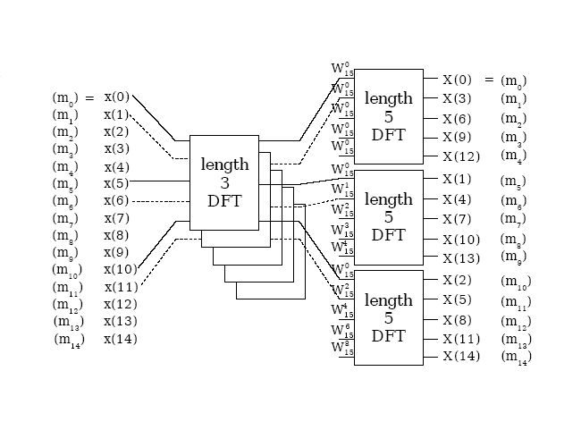 (b) Time-reversed |

Circular convolution is defined as

Circular convolution of two discrete-time signals corresponds to multiplication of their DFTs: (x(n)*h(n) X(k)H(k))
A similar property relates multiplication in time to circular convolution in frequency.

Parseval's theorem relates the energy of a length-N discrete-time signal (or one period) to the energy of its DFT.

The continuous-time Fourier transform, the DTFT, and DFT are all defined as transforms of complex-valued data to complex-valued spectra. However, in practice signals are often real-valued. The DFT of a real-valued discrete-time signal has a special symmetry, in which the real part of the transform values are DFT even symmetric and the imaginary part is DFT odd symmetric, as illustrated in the equation and figure below.
x(n)
real
 (This implies
X(0)
,
(This implies
X(0)
,
 are real-valued.)
The Discrete-Time Fourier Transform (DTFT) is the primary theoretical tool for understanding the frequency content of a discrete-time (sampled) signal. The DTFT is defined as

The inverse DTFT (IDTFT) is defined by an integral formula, because it operates on a continuous-frequency DTFT spectrum:
The DTFT is very useful for theory and analysis, but is not practical for numerically computing a spectrum digitally, because
infinite time samples means
infinite computation
infinite delay
The transform is continuous in the discrete-time frequency, ω
For practical computation of the frequency content of real-world signals, the Discrete Fourier Transform (DFT) is used.
The DFT transforms N samples of a discrete-time signal to the same number of discrete frequency samples, and is defined as
The DFT is invertible by the inverse discrete Fourier transform (IDFT):

The DFT and IDFT are a self-contained, one-to-one transform pair for a length-N discrete-time signal. (That is, the DFT is not merely an approximation to the DTFT as discussed next.) However, the DFT is very often used as a practical approximation to the DTFT.
The DFT gives the discrete-time Fourier series coefficients of a periodic sequence ( x(n)=x(n+N) ) of period N samples, or

as can easily be confirmed by computing the inverse DTFT of the corresponding line spectrum:

The DFT can thus be used to exactly compute the relative values of the N line spectral components of the DTFT of any periodic discrete-time sequence with an integer-length period.
When a discrete-time sequence happens to equal zero for all samples except for those between 0 and N−1,
the infinite sum in the DTFT equation becomes the same as the finite sum from 0 to N−1
in the DFT equation.
By matching the arguments in the exponential terms, we observe that the
DFT values exactly equal the DTFT for specific DTFT frequencies
 .
That is, the DFT computes exact samples of the DTFT at N equally spaced frequencies
.
That is, the DFT computes exact samples of the DTFT at N equally spaced frequencies
 ,
or
,
or

In most cases, the signal is neither exactly periodic nor truly of finite length;
in such cases, the DFT of a finite block of N
consecutive discrete-time samples does not exactly equal
samples of the DTFT at specific frequencies.
Instead, the DFT gives frequency
samples of a windowed (truncated) DTFT
where
Once again,
X(k)
exactly equals
X(ωk)
a DTFT frequency sample only when
x(n)=0 ,
n∉[0, N−1]
The goal of spectrum analysis is often to determine the frequency content of an analog (continuous-time) signal; very often, as in most modern spectrum analyzers, this is actually accomplished by sampling the analog signal, windowing (truncating)
the data, and computing and plotting the magnitude of its DFT.
It is thus essential to relate the DFT frequency samples back to the original analog frequency.
Assuming that the analog signal is bandlimited and the sampling frequency exceeds twice that limit so that no frequency aliasing occurs, the relationship between
the continuous-time Fourier frequency Ω (in radians) and the
DTFT frequency ω imposed by sampling is
ω=ΩT
where T is the sampling period.
Through the relationship
between the DTFT frequency ω
and the DFT frequency index k, the correspondence between the DFT frequency index and the original analog frequency can be found:
 or in terms of analog frequency f in Hertz
(cycles per second rather than radians)
or in terms of analog frequency f in Hertz
(cycles per second rather than radians)
 for k in the range
k
between 0 and
for k in the range
k
between 0 and
 .
It is important to note that
.
It is important to note that
 correspond to negative
frequencies due to the periodicity of the DTFT and the DFT.
correspond to negative
frequencies due to the periodicity of the DTFT and the DFT.
In general, will DFT frequency values
X(k)
exactly equal samples
of the analog Fourier transform
Xa
at the corresponding frequencies?
That is, will
 ?
?
In general, NO. The DTFT exactly corresponds to the continuous-time Fourier transform only when the signal is bandlimited and sampled at more than twice its highest frequency. The DFT frequency values exactly correspond to frequency samples of the DTFT only when the discrete-time signal is time-limited. However, a bandlimited continuous-time signal cannot be time-limited, so in general these conditions cannot both be satisfied.
It can, however, be true for a small class of analog signals which are not time-limited
but happen to exactly equal zero at all sample times outside of the interval
 .
The sinc function with a bandwidth equal to the Nyquist frequency and centered at
t=0
is an example.
.
The sinc function with a bandwidth equal to the Nyquist frequency and centered at
t=0
is an example.
If more than N equally spaced frequency samples of
a length-N signal are desired, they can easily be obtained
by zero-padding the discrete-time signal and computing a DFT of the
longer length.
In particular, if
LN
DTFT samples are desired
of a length-N sequence, one can compute the length-
LN
DFT of a
length-
LN
zero-padded
sequence

 Note that
zero-padding interpolates the spectrum. One
should always zero-pad (by about at least a factor of 4) when
using the DFT to approximate
the DTFT to get a clear
picture of the DTFT.
While performing computations on zeros may at first seem inefficient,
using
Note that
zero-padding interpolates the spectrum. One
should always zero-pad (by about at least a factor of 4) when
using the DFT to approximate
the DTFT to get a clear
picture of the DTFT.
While performing computations on zeros may at first seem inefficient,
using