Digital filters with an Infinite-duration Impulse Response (IIR) have characteristics that make them useful in many applications. This section develops and discusses the properties and characteristics of these filters3.
Because of the feedback necessary in an implementation, the Infinite Impulse Response (IIR) filter is also called a recursive filter or, sometimes, an autoregressive moving-average filter (ARMA). In contrast to the FIR filter with a polynomial transfer function, the IIR filter has a rational transfer function. The transfer function being a ratio of polynomials means it has finite poles as well as zeros, and the frequency-domain design problem becomes a rational-function approximation problem in contrast to the polynomial approximation for the FIR filter4. This gives considerably more flexibility and power, but brings with it certain problems in both design and implementation3, 2, 1.
The defining relationship between the input and output variables for the IIR filter is given by

The second summation in Equation 3.1 is exactly the same moving average of the present plus past M values of the input that occurs in the definition of the FIR filter. The difference arises from the first summation, which is a weighted sum of the previous N output values. This is the feedback or recursive part which causes the response to an impulse input theoretically to endure forever. The calculation of each output term y(n) from Equation 3.1 requires N+M+1 multiplications and N+M additions. There are other algorithms or structures for calculating y(n) that may require more or less arithmetic.
In addition to the number of calculations required to calculate each output term being a measure of efficiency, the amount of storage for coefficients and intermediate calculations is important. DSP chips are designed to efficiently implement calculations such as Equation 3.1 by having a single cycle operation that multiplies a variable by a constant and accumulates it. In parallel with that operation, it is simultaneously calculating the address of the next variable.
Just as in the case of the FIR filter, the output of an IIR filter can also be calculated by convolution.

In this case, the duration of the impulse response h(n) is infinite and, therefore, the number of terms in Equation 3.2 is infinite. The N+M+1 operations required in Equation 3.1 are clearly preferable to the infinite number required by Equation 3.2. This gives a hint as to why the IIR filter is very efficient. The details will become clear as the characteristics of the IIR filter are developed in this section.
The transfer function of a filter is defined as the ratio Y(z)/X(z), where Y(z) and X(z) are the z-transforms of the output y(n) and input x(n), respectively. It is also the z-transform of the impulse response. Using the definition of the z-transform in Equation 32 from Discrete-Time Signals, the transfer function of the IIR filter defined in Equation 3.1 is

This transfer function is also the ratio of the z-transforms of the a(n) and b(n) terms.

The frequency response of the filter is found by setting z=ejω, which gives Equation 3.1 the form

It should be recalled that this form assumes a
sampling rate of T=1. To simplify notation, H(ω) is used
to denote the frequency response rather than  .
.
This frequency-response function is complex-valued and consists of a magnitude and phase. Even though the impulse response is a function of the discrete variable n, the frequency response is a function of the continuous-frequency variable ω and is periodic with period 2π.
Unlike the FIR filter case, exactly linear phase is impossible for the IIR filter. It has been shown that linear phase is equivalent to symmetry of the impulse response. This is clearly impossible for the IIR filter with an impulse response that is zero for n<0 and nonzero for n going to infinity.
The FIR linear-phase filter allowed removing the phase from the design process. The resulting problem was a real-valued approximation problem requiring the solution of linear equations. The IIR filter design problem is more complicated. Linear phase is not possible, and the equations to be solved are generally nonlinear. The most common technique is to approximate the magnitude of the transfer function and let the phase take care of itself. If the phase is important, it becomes part of the approximation problem, which then is often difficult to solve.
As shown in another module, L equally spaced samples of H(ω) can be approximately calculated by taking an L-length DFT of h(n) given in Equation 3.5. However, unlike for the FIR filter, this requires that the infinitely long impulse response be truncated to at least length-L. A more satisfactory alternative is to use the DFT to evaluate the numerator and denominator of Equation 3.4 separately rather than to approximately evaluate Equation 3.5. This is accomplished by appending L–N zeros to the a(n) and L–M zeros to the b(n) from Equation 3.1, and taking length-L DFTs of both to give

where the division is a term-wise division of each of the L values of the DFTs as a function of k. This direct method of calculation is a straightforward and flexible technique that does not involve truncation of h(n) and the resulting error. Even nonuniform spacing of the frequency samples can be achieved by altering the DFT as was suggested for the FIR filter. Because IIR filters are generally lower in order than FIR filters, direct use of the DFT is usually efficient enough and use of the FFT is not necessary. Since the a(n) and b(n) do not generally have the symmetries of the FIR h(n), the DFTs cannot be made real and, therefore, the shifting and stretching techniques of other modules are not applicable.
As an example, the frequency-response plot of a third-order elliptic-function lowpass filter with a transfer function of

is given in Figure 3.1a. The details for designing this filter are discussed in elsewhere. A similar performance for the magnitude response would require a length of 18 for a linear-phase FIR filter.
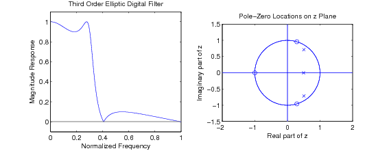
The possible locations of the zeros of the transfer function of an FIR linear-phase filter were analyzed elsewhere. For the IIR filter, there are poles as well as zeros. For most applications, the coefficients a(n) and b(n) are real and, therefore, the poles and zeros occur in complex conjugate pairs or are real. A filter is stable if for any bounded input, the output is bounded. This implies the poles of the transfer function must be strictly inside the unit circle of the complex z plane. Indeed, the possibility of an unstable filter is a serious problem in IIR filter design, which does not exist for FIR filters. An important characteristic of any design procedure is the guarantee of stable designs, and an important ability in the analysis of a given filter is the determination of stability. For a linear filter analysis, this involves the zeros of the denominator polynomial of Equation 3.4. The location of the zeros of the numerator, which are the zeros of H(z), are important to the performance of the filter, but have no effect on stability.
If both the poles and zeros of a transfer function are all inside or on the unit circle of the z-plane, the filter is called minimum phase. The effects of a pole or zero at a radius of r from the origin of the z-plane on the magnitude of the transfer function are exactly the same as one at the same angle but at a radius of 1/r. However, the effect on the phase characteristics is different. Since only stable filters are generally used in practice, all the poles must be inside the unit circle. For a given magnitude response, there are two possible locations for each zero that is not on the unit circle. The location that is inside gives the least phase shift, hence the name “minimum- phase" filter.
The locations of the poles and zeros of the example in Equation 3.7 are given in Figure 3.1b.
Since evaluating the frequency response of a transfer function is the same as evaluating H(z) around the unit circle in the z-plane, a comparison of the frequency-response plot in Figure 3.1a and the pole-zero locations in Figure 3.1b gives insight into the effects of pole and zero location on the frequency response. In the case where it is desirable to reject certain bands of frequencies, zeros of the transfer function will be located on the unit circle at locations corresponding to those frequencies.
By having both poles and zeros to describe an IIR filter, much more can be done than in the FIR filter case where only zeros exist. Indeed, an FIR filter is a special case of an IIR filter with a zero-order denominator. This generality and flexibility does not come without a price. The poles are more difficult to realize than the zeros, and the design is more complicated.
This section has given the basic definition of the IIR or recursive digital filter and shown it to a generalization of the FIR filter described in the previous chapters. The feedback terms in the IIR filter cause the transfer function to be a rational function with poles as well as zeros. This feedback and the resulting poles of the transfer function give a more versatile filter requiring fewer coefficients to be stored and less arithmetic. Unfortunately, it also destroys the possibility of linear phase and introduces the possibility of instability and greater sensitivity to the effects of quantization. The design methods, which are more complicated than for the FIR filter, are discussed in another section, and the implementation, which also is more complicated, is discussed in still another section.
Mitra, Sanjit K. (2006). Digital Signal Processing, A Computer-Based Approach. (Third). [First edition in 1998, second in 2001]. New York: McGraw-Hill.
Oppenheim, A. V. and Schafer, R. W. (1999). Discrete-Time Signal Processing. (Second). [Earlier editions in 1975 and 1989]. Englewood Cliffs, NJ: Prentice-Hall.
Parks, T. W. and Burrus, C. S. (1987). Digital Filter Design. New York: John Wiley & Sons.
Rader, Charles M. (2006, November). The Rise and Fall of Recursive Digital Filters. IEEE Signal Processing Magazine, 23(6), 46–49.
The design of a digital filter is usually specified in terms of the characteristics of the signals to be passed through the filter. In many cases, the signals are described in terms of their frequency content. For example, even though it cannot be predicted just what a person may say, it can be predicted that the speech will have frequency content between 300 and 4000 Hz. Therefore, a filter can be designed to pass speech without knowing what the speech is. This is true of many signals and of many types of noise or interference. For these reasons among others, specifications for filters are generally given in terms of the frequency response of the filter.
The basic IIR filter design process is similar to that for the FIR problem:
Choose a desired response, usually in the frequency domain;
Choose an allowed class of filters, in this case, the Nth-order IIR filters;
Establish a measure of distance between the desired response and the actual response of a member of the allowed class; and
Develop a method to find the best allowed filter as measured by being closest to the desired response.
This section develops several practical methods for IIR filter design. A very important set of methods is based on converting Butterworth, Chebyshev I and II, and elliptic-function analog filter designs to digital filter designs by both the impulse- invariant method and the bilinear transformation. The characteristics of these four approximations are based on combinations of a Taylor's series and a Chebyshev approximation in the pass and stopbands. Many results from this chapter can be used for analog filter design as well as for digital design.
Extensions of the frequency-sampling and least-squared-error design for the FIR filter are developed for the IIR filter. Several direct iterative numerical methods for optimal approximation are described in this chapter. Prony's method and direct numerical methods are presented for designing IIR filters according to time-domain specifications.
The discussion of the four classical lowpass filter design methods is arranged so that each method has a section on properties and a section on design procedures. There are also design programs in the appendix. An experienced person can simply use the design programs. A less experienced designer should read the design procedure material, and a person who wants to understand the theory in order to modify the programs, develop new programs, or better understand the given ones, should study the properties section and consult the references.
The mathematical problem inherent in the frequency-domain filter design problem is the approximation of a desired complex frequency-response function Hd(z) by a rational transfer function H(z) with an Mth-degree numerator and an Nth-degree denominator for values of the complex variable z along the unit circle of z=ejω. This approximation is achieved by minimizing an error measure between H(ω) and Hd(ω).
For the digital filter design problem, the mathematics are complicated by the approximation being defined on the unit circle. In terms of z, frequency is a polar coordinate variable. It is often much easier and clearer to formulate the problem such that frequency is a rectangular coordinate variable, in the way it naturally occurs for analog filters using the Laplace complex variable s. A particular change of complex variable that converts the polar coordinate variable to a rectangular coordinate variable is the bilinear transformation4, 5, 3, 2.

The details of the bilinear and alternative transformations are covered elsewhere. For the purposes of this section, it is sufficient to observe4, 3 that the frequency response of a filter in terms of the new variable is found by evaluating H(s) along the imaginary axis, i.e., for s=jω. This is exactly how the frequency response of analog filters is obtained.
There are two reasons that the approximation process is often formulated in terms of the square of the magnitude of the transfer function, rather than the real and/or imaginary parts of the complex transfer function or the magnitude of the transfer function. The first reason is that the squared-magnitude frequency- response function is an analytic, real-valued function of a real variable, and this considerably simplifies the problem of finding a “best" solution. The second reason is that effects of the signal or interference are often stated in terms of the energy or power that is proportional to the square of the magnitude of the signal or noise.
In order to move back and forth between the transfer function F(s) and the squared-magnitude frequency response |F(jω)|2, an intermediate function is defined. The analytic complex-valued function of the complex variable s is defined by
which is related to the squared magnitude by