There are two types of linear, time-invariant digital filters. We will investigate digital filters with a finite-duration impulse response (FIR) in this section and those with an infinite-duration impulse response (IIR) in another document. FIR filters have characteristics that make them useful in many applications 3, 2.
FIR filters can achieve an exactly linear phase frequency response
FIR filters cannot be unstable.
FIR filters are generally less sensitive to coefficient round-off and finite-precision arithmetic than IIR filters.
FIR filters design methods are generally linear.
FIR filters can be efficiently realized on general or special-purpose hardware.
However, frequency responses that need a rapid transition between bands and do not require linear phase are often more efficiently realized with IIR filters.
It is the purpose of this section to examine and evaluate these characteristics which are important in the design of the four basic types of linear-phase FIR filters.
Because of the usual methods of implementation, the Finite Impulse Response (FIR) filter is also called a nonrecursive filter or a convolution filter. From the time-domain view of this operation, the FIR filter is sometimes called a moving-average or running-average filter. All of these names represent useful interpretations that are discussed in this section; however, the name, FIR, is most commonly seen in filter-design literature and is used in these notes.
The duration or sequence length of the impulse response of these filters is by definition finite; therefore, the output can be written as a finite convolution sum by

where n and m are integers, perhaps representing samples in time, and where x(n) is the input sequence, y(n) the output sequence, and h(n) is the length-N impulse response of the filter. With a change of index variables, this can also be written as

If the FIR filter is interpreted as an extension of a moving sum or as a weighted moving average, some of its properties can easily be seen. If one has a sequence of numbers, e.g., prices from the daily stock market for a particular stock, and would like to remove the erratic variations in order to discover longer term trends, each number could be replaced by the average of itself and the preceding three numbers, i.e., the variations within a four-day period would be “averaged out" while the longer-term variations would remain. To illustrate how this happens, consider an artificial signal x(n) containing a linear term, K1n, and an undesired oscillating term added to it, such that

If a length-2 averaging filter is used with

it can be verified that, after two outputs, the output y(n) is exactly the linear term x(n) with a delay of one half sample interval and no oscillation.
This example illustrates the basic FIR filter-design problem: determine N, the number of terms for h(n), and the values of h(n) for achieving a desired effect on the signal. The reader should examine simple examples to obtain an intuitive idea of the FIR filter as a moving average; however, this simple time-domain interpretation will not suffice for complicated problems where the concept of frequency becomes more valuable.
The output of a length-N FIR filter can be calculated from the input using convolution.

and the transfer function of an FIR filter is given by the z-transform of the finite length impulse response h(n) as

The frequency response of a filter, is found by setting z=ejω, which is the same as the discrete-time Fourier transform (DTFT) of h(n), which gives

with ω being frequency in radians per second.
Strictly speaking, the exponent should be –jωTn where T is the
time interval between the integer steps of n (the sampling interval).
But to simplify notation, it will be assumed that T=1 until later in the
notes where the relation between n and time is more important. Also to
simplify notation, H(ω) is used to represent the frequency response
rather that  . It should always be clear from the context
whether H is a function of z or ω.
. It should always be clear from the context
whether H is a function of z or ω.
This frequency-response function is complex-valued and consists of a magnitude and a phase. Even though the impulse response is a function of the discrete variable n, the frequency response is a function of the continuous-frequency variable ω and is periodic with period 2π. This periodicity is easily shown by

with frequency denoted by ω in radians per second or by f in Hz (hertz or cycles per second). These are related by

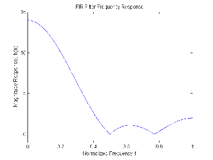
An example of a length-5 filter might be

with a frequency-response plot shown over the base frequency band (0<ω<π or 0<f<1 in Figure 2.1. To illustrate the periodic nature of the total frequency response, Figure 2.2 shows the response over a wider set of frequencies.

The Discrete Fourier Transform (DFT) can be used to evaluate the frequency response at certain frequencies. The DFT 1 of the length-N impulse response h(n) is defined as

which, when compared to Equation 2.7, gives

for ωk=2πk/N.
This states that the DFT of h(n) gives N samples of the frequency-response function H(ω). This sampling at N points may not give enough detail, and, therefore, more samples are needed. Any number of equally spaced samples can be found with the DFT by simply appending L–N zeros to h(n) and taking an L-length DFT. This is often useful when an accurate picture of all of H(ω) is required. Indeed, when the number of appended zeros goes to infinity, the DFT becomes the discrete-time Fourier transform of h(n).
The fact that the DFT of h(n) is a set of N samples of the frequency response suggests a method of designing FIR filters in which the inverse DFT of N samples of a desired frequency response gives the filter coefficients h(n). That approach is called frequency sampling and is developed in another section.
A particular property of FIR filters that has proven to be very powerful is that a linear phase shift for the frequency response is possible. This is especially important to time domain details of a signal. The spectrum of a signal contains the individual frequency domain components separated in frequency. The process of filtering usually involves passing some of these components and rejecting others. This is done by multiplying the desired ones by one and the undesired ones by zero. When they are recombined, it is important that the components have the same time domain alignment as they originally did. That is exactly what linear phase insures. A phase response that is linear with frequency keeps all of the frequency components properly registered with each other. That is especially important in seismic, radar, and sonar signal analysis as well as for many medical signals where the relative time locations of events contains the information of interest.
To develop the theory for linear phase FIR filters, a careful definition of phase shift is necessary. If the real and imaginary parts of H(ω) are given by

where  and the magnitude is defined
by
and the magnitude is defined
by

and the phase by

which gives

in terms of the magnitude and phase. Using the real and imaginary parts is using a rectangular coordinate system and using the magnitude and phase is using a polar coordinate system. Often, the polar system is easier to interpret.
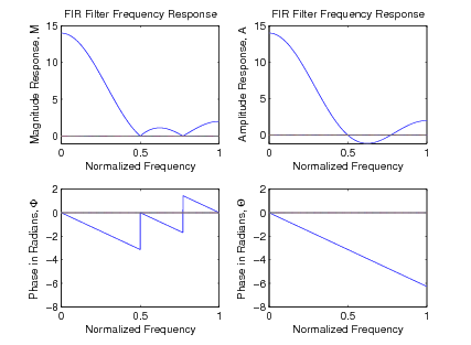
Mathematical problems arise from using |H(ω)| and Φ(ω), because |H(ω)| is not analytic and Φ(ω) not continuous. This problem is solved by introducing an amplitude function A(ω) that is real valued and may be positive or negative. The frequency response is written as

where A(ω) is called the amplitude in order to distinguish it from the magnitude |H(ω)|, and Θ(ω) is the continuous version of Φ(ω). A(ω) is a real, analytic function that is related to the magnitude by

or

With this definition, A(ω) can be made analytic and Θ(ω) continuous. These are much easier to work with than |H(ω)| and Φ(ω). The relationship of A(ω) and |H(ω)|, and of Θ(ω) and Φ(ω) are shown in Figure 2.3.
To develop the characteristics and properties of linear-phase filters, assume a general linear plus constant form for the phase function as

This gives the frequency response function of a length-N FIR filter as

and

Equation 2.22 can be put in the form of

if M (not necessarily an integer) is defined by

or equivalently,

Equation 2.22 then becomes

There are two possibilities for putting this in the form of Equation 2.23 where A(ω) is real: K1=0 or K1=π/2. The first case requires a special even symmetry in h(n) of the form

which gives

where A(ω) is the amplitude, a real-valued function of ω and e–jMω gives the linear phase with M being the group delay. For the case where N is odd, using Equation 2.26, Equation 2.27, and Equation 2.28, we have

or with a change of variables,

which becomes

where  is a shifted h(n).
These formulas can be made simpler by defining new coefficients so that
Equation 2.29 becomes
is a shifted h(n).
These formulas can be made simpler by defining new coefficients so that
Equation 2.29 becomes

where

and Equation 2.31 becomes

wit