j
(20)
3. Compute the filter gain:
T
1
K
P ( k 1| k) C ( k 1)
j
j
j
S−
=
+
+
j (21)
Step 2.2: Correction step
Update the estimated state and covariance matrix:
ˆ x ( k + 1| k + 1) = ˆ x ( k + 1| k) +
j
j
Kjrj (22)
P ( k + 1| k + 1) = P ( k + 1| k)
T
−
j
j
KjSjKj (23)
Step 3. Updating the model probability
The model probability is an important parameter for the system fault detection and
diagnosis. For this, a likelihood function should be defined in advance, and then the model
probability be updated based on the likelihood function.
1. Compute the likelihood function:
1
⎡ 1
⎤
T
1
L ( k + 1) =
exp
−
−
j
r S r
⎢
(24)
⎣ 2 j j j ⎥
2π S
⎦
j
2. Update the model probability:
μ ( k + 1| k) L ( k + 1)
μ ( k + 1)
j
j
=
j
(25)
N
∑ μ ( k + 1| k) L ( k + 1)
=1 j
j
j
Step 4. Fault detection and diagnosis
G
1. Define the model probability vector μ( k + 1) = [μ
+
μ
+
μ
+
1( k
1), 2( k 1),...,
( k 1)]
N
. The
maximum value of the model probability vector for FDD can be obtained as
Fuzzy Logic Based Interactive Multiple Model Fault Diagnosis for PEM Fuel Cell Systems
431
G
μ
=
μ +
FDDmax
max ( k 1) (26)
The index of the maximum value of the model probability vector component can be
determined as
G
j = find(μ
== μ +
FDDmax
( k 1)) (27)
2. Fault decision–FDD logic
The mode probabilities provide an indication of mode in effect at the current sampling
period. Hence, it is natural to be used as an indicator of a failure. According to the
information provided by the model probability, both fault detection and diagnosis can be
achieved. The fault decision can be determined by
⎧≥ μ ⇒
⎪
H : Delare fault corresponding to j th mode
T
j
μFDDmax ⎨
(28)
⎪< μ ⇒
⎩
T
H 1 : No fault
Or alternatively,
'
μ
⎧≥ μ ⇒
⎪
H : Delare fault corresponding to j th mode
FDDmax
T
j
(29)
μG
⎨
+
'
max ( k 1) ⎪< μ ⇒
≠
⎩
T
H 1 : No fault
i j
Step 5. Estimate fusion and combination that yields the overall state estimate as the
probabilistically weighted sum of the updated state estimates of all the filters. The
probability of a mode in effect plays a key role in determining the weights
associated with the fusion of state estimates and covariances. The estimates and
covariance matrices can be obtained as:
N
ˆ(
x k + 1| k + 1) =
ˆ
∑ x ( k + 1| k + 1)μ ( k + 1)
j
j
(30)
j=1
P( k + 1| k + 1) =
N
= ∑
(31)
[ P ( k| k) + ( ˆ(
x k + 1| k + 1) − ˆ x ( k + 1| k + 1))( ˆ(
x k + 1| k + 1) − ˆ x ( k + 1| k + 1)) T ]μ ( k + 1)
j
j
j
j
j=1
It will be seen from Section 4 that the transition probability plays an important role in the
IMM approach to FDD. In this study, the transition probability is adapted online through
the Takagi-Sugeno fuzzy logic (Takagi & Sugeno, 1985). The overall framework of the
proposed fuzzy logic based IMM FDD algorithm is illustrated in Fig. 1.
It is worth noting that decision rule (28) or (29) provides not only fault detection but also the
information of the type (sensor or actuator), location (which sensor or actuator), size (total
failure or partial fault with the fault magnitude) and fault occurrence time, that is,
simultaneous detection and diagnosis. For partial faults, the magnitude (size) can be
determined by the probabilistically weighted sum of the fault magnitudes of the
corresponding partial fault models. Another advantage of the IMM approach is that FDD is
integrated with state estimation. The overall estimate provides the best state estimation of
the system subject to failures. Furthermore, unlike other observer-based or Kalman filter
432
Discrete Time Systems
based approaches, there is no extra computation for the fault decision because the mode
probabilities are necessary in the IMM algorithm. Furthermore, the overall estimate is
generated by the probabilistically weighted sum of estimates from the single-model-based
filters. Therefore, it is better and more robust than any single-model-based estimate. This
state estimate does not depend upon the correctness of fault detection and in fact, the
accurate state estimation can facilitate the correct FDD. The detection threshold μT is
universal in the sense that it does not depend much on the particular problem at hand and a
robust threshold can be determined easily. In other words, the FDD performance of the
IMM approach varies little in most cases with respect to the choice of this threshold (Zhang
& Li, 1998). On the other hand, the residual-based fault detection logic relies heavily on the
threshold used, which is problem-relevant. Quite different detection thresholds have to be
used for FDD problems of different systems and design of such a threshold is not trivial.
Moreover, without comparing with the threshold, the value of the measurement residual
itself does not provide directly meaningful detection and indication of the fault situations.
z( k + )
1
ˆ
ˆ
x ( k | k)
x ( k +1| k + )
1
N
1
P ( k | k)
Filter 1
P ( k +1| k + )
1
N
1
r 1
ˆ
ˆ
x ( k | k)
x ( k +1| k + )
1
2
2
P ( k | k)
Filter 2
P ( k +1| k + )
1
2
2
r 2
#
Interaction
#
#
ˆ x ( k | k)
ˆ x ( k +1| k + )
1
N
2
Filter N
P ( k | k)
P ( k +1| k + )
1
2
N
rN
μ
μ
1
1
μ
μ
ˆ x( k +1| k + )
1
2
2
Fuzzy logic based model
Estimation
"
probability update
"
fusion
P( k +1| k + )
1
μ N
μ
μ
μ
" μ
N
1
2
N
μ
{
max
}> μ
j
T
Fault
j
?
Decision
Fig. 1. Block diagram of the proposed fuzzy logic based IMM FDD approach
3. Update of transition probability by fuzzy logic
As aforementioned, the transition probability plays an important role in interacting and
mixing the information of each individual filter. However, an assumption that the transition
probability is constant over the total period of FDD can lead to some problems. Even if the
fault tolerant control treats the first failure successfully, the unchanged transition probability
Fuzzy Logic Based Interactive Multiple Model Fault Diagnosis for PEM Fuel Cell Systems
433
can mislead the FDD to intermittently declare a false failure alarm. This is because the fact
that the normal mode before the first failure occurrence is not the normal mode any longer.
The declared fault mode should be changed to a new normal mode after the first failure. On
that account, the fuzzy-tuning algorithm of the transition probability is proposed in this
study.
The transition probability from any particular failure mode to the normal mode is generally
set larger than others in order to prevent a false fault diagnosis. However, it may have a bad
influence on performing correct fault diagnosis because the model probability of the healthy
mode tends to increase again as the current failed system converges to the steady state by
the fault tolerant control law even after a fault occurs. This problem can be overcome by
adjusting the transition probability after the fault occurrence. For example, if the model
probability of a certain failure mode remains larger than that of any other mode for an
assigned time, the transition probability related to the corresponding failure mode should be
increased. On the other hand, the transition probability related to the previous mode should
be decreased to reflect the fact that the failed mode selected by the fault decision algorithm
becomes currently dominant. In this work, the fuzzy-tuning algorithm is adopted to adjust
the transition probabilities effectively.
Now introduce a determination variable Ci which decides whether or not the transition
probabilities should be adjusted. First, the initial value of each mode’s determination
variable is set to zero. The increment of the determination variable can be obtained through
the fuzzy logic with inputs composed of the model probabilities at every step. If the
determination variable Ci of a certain mode exceeds a predefined threshold value CT, then
the transition probabilities are adjusted, and the determination value of each mode is
initialized. The overall process is illustrated in Fig. 2.
3.1 Fuzzy input
A fuzzy input for adjusting transition probabilities includes the model probabilities from the
IMM filter. At each sampling time, the model probabilities of every individual filter are
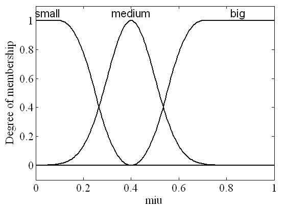
transmitted to the fuzzy system. In this work, the membership function is designed as in
Fig. 3 for the fuzzy input variables “small,” “medium,” and “big” representing the relative
size of the model probability.
3.2 Fuzzy rule
The T-S fuzzy model is used as the inference logic in this work. The T-S fuzzy rule can be
represented as
If
χ is A and ξ is B then Ζ = f( χ , ξ ) (32)
where A and B are fuzzy sets, and Ζ = f( χ , ξ ) is a non-fuzzy function. The fuzzy rule of
adjusting transition probabilities is defined using the T-S model as follows
If μ is small, then
s
C
Δ
= 0
j
j
If μ is medium, then
m
C
Δ
= 0.5
j
j
(33)
If μ is big, then
b
C
Δ
= 1
j
j
434
Discrete Time Systems
Start
k← k+1
Ci( k)=0
Update Ci( k+1) using TS
fuzzy logic
Ci( k+1)= Ci( k)+△ Ci( k+1)
No
Ci( k+1) CT
Yes
πij← πij _new
Fig. 2. Flowchart of T-S fuzzy logic for adaptive model probability update
Fig. 3. Fuzzy membership function
Fuzzy Logic Based Interactive Multiple Model Fault Diagnosis for PEM Fuel Cell Systems
435
3.3 Fuzzy output
The output of the fuzzy system using the T-S model can be obtained by the weighted
average using a membership degree in a particular fuzzy set as follows:
s
s
m
m
b
b
w C
Δ
+ w C
Δ
+ w C
Δ
C
Δ ( k)
j
j
j
j
j
j
=
j
(34)
s
m
b
w +
+
j
wj wj
where
s
wj , m
wj , and b
wj is the membership degree in the j th mode for group small,
medium, and big, respectively. During the monitoring process, the determination variable
of the j th mode is accumulated as
C
Δ ( k + 1) = C ( k) + C
Δ ( k + 1)
j
j
j
(35)
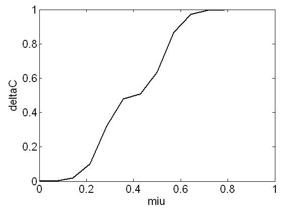
The designed fuzzy output surface of the T-S fuzzy interference system is shown in Fig. 4.
Fig. 4. Output surface of the fuzzy interference system
Once the determination variable of a certain fault mode exceeds the threshold value T
C ,
then all the elements of the transition probability matrix from the other modes to the
corresponding fault mode are increased.
3.4 Transition probability design
The diagonal elements of the transition probability matrix can be designed as follows
(Zhang & Li, 1998).
⎧
T ⎫
⎪
⎪
π = max⎨ l ,1 −
jj
j
(36)
τ ⎬
⎪⎩
j ⎪
⎭
where T , τ j , and lj are the sampling time, the expected sojourn time, and the predefined
threshold of the transition probability, respectively. For example, the “normal-to-normal’’
436
Discrete Time Systems
transition probability, π
π = −
τ
τ
11 , can be obtained by 11
1 T / 1 (here 1 denotes the mean
time between failures) since T is much smaller than τ1 in practice. The transition probability
from the normal mode to a fault mode sums up to 1 − π11 . To which particular fault mode it
jumps depends on the relative likelihood of the occurrence of the fault mode. While in
reality mean sojourn time of total failures is the down time of the system, which is usually
large and problem-dependent, to incorporate various fault modes into one sequence for a
convenient comparison of different FDD approaches, the sojourn time of the total failures is
assumed to be the same as that of the partial faults in this work.
“Fault-to-fault’’ transitions are normally disallowed except in the case where there is sufficient
prior knowledge to believe that partial faults can occur one after another. Hence, by using (36),
the elements of the transition probability related to the current model can be defined by
T
1 − p
p = 1 −
n
=
n
, p
(37)
τ
n
−
n
N 1
T
p = 1 −
= −
f
, p
1 p (38)
τ
f
f
f
where pn and pf are the diagonal elements of the normal and failure mode, respectively,
and p n and p f are off-diagonal elements to satisfy the constraint that all the row sum of the
transition probability matrix should be equal to one. In addition, N is the total number of the
assumed models, and τ
τ
n and f are the expected sojourn times of the normal and failure
mode, respectively.
After a failure declaration by the fuzzy decision logic, the transition probability from the
other modes to the corresponding failure model (say the m th mode) should be increased,
whereas the transition probabilities related to the nonfailed model should be relatively
decreased. For this purpose, the transition probability matrix of each mode is set as
follows.
⎧ p , = =
n
i j