Conditional expectation, given a random vector, plays a fundamental role in much of modern probability theory. Various types of “conditioning” characterize some of the more important random sequences and processes. The notion of conditional independence is expressed in terms of conditional expectation. Conditional independence plays an essential role in the theory of Markov processes and in much of decision theory.
We first consider an elementary form of conditional expectation with respect to an event. Then we consider two highly intuitive special cases of conditional expectation, given a random variable. In examining these, we identify a fundamental property which provides the basis for a very general extension. We discover that conditional expectation is a random quantity. The basic property for conditional expectation and properties of ordinary expectation are used to obtain four fundamental properties which imply the “expectationlike” character of conditional expectation. An extension of the fundamental property leads directly to the solution of the regression problem which, in turn, gives an alternate interpretation of conditional expectation.
If a conditioning event C occurs, we modify the original probabilities by introducing the conditional probability measure P(·|C). In making the change from

we effectively do two things:
We limit the possible outcomes to event C
We “normalize” the probability mass by taking P(C) as the new unit
It seems reasonable to make a corresponding modification of mathematical expectation when the occurrence of event C is known. The expectation E[X] is the probability weighted average of the values taken on by X. Two possibilities for making the modification are suggested.
We could replace the prior probability measure P(·) with the conditional probability measure P(·|C) and take the weighted average with respect to these new weights.
We could continue to use the prior probability measure P(·) and modify the averaging process as follows:
Consider the values X(ω) for only those ω∈C. This may be done
by using the random variable ICX which has value X(ω) for ω∈C and
zero elsewhere. The expectation  is the probability weighted sum of
those values taken on in C.
is the probability weighted sum of
those values taken on in C.
The weighted average is obtained by dividing by P(C).
These two approaches are equivalent. For a simple random variable  in canonical form

The final sum is expectation with respect to the conditional probability measure. Arguments using basic theorems on expectation and the approximation of general random variables by simple random variables allow an extension to a general random variable X. The notion of a conditional distribution, given C, and taking weighted averages with respect to the conditional probability is intuitive and natural in this case. However, this point of view is limited. In order to display a natural relationship with more the general concept of conditioning with repspect to a random vector, we adopt the following
Definition. The conditional expectation of X, given event C with positive probability, is the quantity

Remark. The product form  is often useful.
Suppose X∼ exponential (λ) and C={1/λ≤X≤2/λ}. Now IC=IM(X) where  .
.


Thus

Suppose  and
and  in canonical form. We suppose
 and
and  , for each permissible i,j. Now

We take the expectation relative to the conditional probability  to get

Since we have a value for each ti in the range of X, the function e(·) is defined on the range of X. Now consider any reasonable set M on the real line and determine the expectation


We have the pattern

for all ti in the range of X.
We return to examine this property later. But first, consider an example to display the nature of the concept.
Suppose the pair  has the joint distribution


| 0 | 1 | 4 | 9 |
| Y = 2 | 0.05 | 0.04 | 0.21 | 0.15 |
| 0 | 0.05 | 0.01 | 0.09 | 0.10 |
| -1 | 0.10 | 0.05 | 0.10 | 0.05 |

| 0.20 | 0.10 | 0.40 | 0.30 |
Calculate  for each possible value ti taken on by X

=(–1·0.10+0·0.05+2·0.05)/0.20=0
E[Y|X=1]=(–1·0.05+0·0.01+2·0.04)/0.10=0.30
E[Y|X=4]=(–1·0.10+0·0.09+2·0.21)/0.40=0.80
E[Y|X=9]=(–1·0.05+0·0.10+2·0.15)/0.10=0.83
The pattern of operation in each case can be described as follows:
For the ith column, multiply each value uj
by  , sum, then divide by
  .
.
The following interpretation helps visualize the conditional expectation and points to an important result in the general case.
For each ti we use the mass distributed “above” it. This mass is distributed along a vertical line at values uj taken on by Y. The result of the computation is to determine the center of mass for the conditional distribution above t=ti. As in the case of ordinary expectations, this should be the best estimate, in the mean-square sense, of Y when X=ti. We examine that possibility in the treatment of the regression problem in the section called “The regression problem”.
Although the calculations are not difficult for a problem of this size, the basic pattern can be implemented simply with MATLAB, making the handling of much larger problems quite easy. This is particularly useful in dealing with the simple approximation to an absolutely continuous pair.
X = [0 1 4 9];             % Data for the joint distribution
Y = [-1 0 2];
P = 0.01*[ 5  4 21 15; 5  1  9 10; 10  5 10  5];
jcalc                      % Setup for calculations
Enter JOINT PROBABILITIES (as on the plane)  P
Enter row matrix of VALUES of X  X
Enter row matrix of VALUES of Y  Y
 Use array operations on matrices X, Y, PX, PY, t, u, and P
EYX = sum(u.*P)./sum(P);   % sum(P) = PX  (operation sum yields column sums)
disp([X;EYX]')             % u.*P = u_j P(X = t_i, Y = u_j) for all i, j
         0         0
    1.0000    0.3000
    4.0000    0.8000
    9.0000    0.8333
The calculations extend to  . Instead of values of uj we use
values of
. Instead of values of uj we use
values of  in the calculations. Suppose Z=g(X,Y)=Y2–2XY.
G = u.^2 - 2*t.*u;         % Z = g(X,Y) = Y^2 - 2XY
EZX = sum(G.*P)./sum(P);   % E[Z|X=x]
disp([X;EZX]')
         0    1.5000
    1.0000    1.5000
    4.0000   -4.0500
    9.0000  -12.8333
Suppose the pair  has joint density function fXY. We seek to use
the concept of a conditional distribution, given X=t. The fact that
P(X=t)=0 for each t requires a modification of the approach adopted in
the discrete case. Intuitively, we consider the conditional density
has joint density function fXY. We seek to use
the concept of a conditional distribution, given X=t. The fact that
P(X=t)=0 for each t requires a modification of the approach adopted in
the discrete case. Intuitively, we consider the conditional density

The condition fX(t)>0 effectively determines the range of X. The function fY|X(·|t) has the properties of a density for each fixed t for which fX(t)>0.

We define, in this case,

The function e(·) is defined for fX(t)>0, hence effectively on the range of X. For any reasonable set M on the real line,


Thus we have, as in the discrete case, for each t in the range of X.

Again, we postpone examination of this pattern until we consider a more general case.
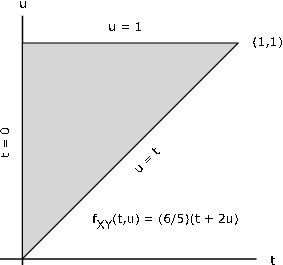
Suppose the pair  has joint density
  on the triangular region bounded by t=0, u=1, and
u=t (see Figure 14.1). Then
on the triangular region bounded by t=0, u=1, and
u=t (see Figure 14.1). Then

By definition, then,

We thus have

Theoretically, we must rule out t=1 since the denominator is zero for that value of t. This causes no problem in practice.
We are able to make an interpretation quite analogous to that for the discrete case. This also points the way to practical MATLAB calculations.
For any