5.1 Continuous Random Variables1
5.1.1 Student Learning Outcomes
By the end of this chapter, the student should be able to:
• Recognize and understand continuous probability density functions in general.
• Recognize the uniform probability distribution and apply it appropriately.
• Recognize the exponential probability distribution and apply it appropriately.
5.1.2 Introduction
Continuous random variables have many applications. Baseball batting averages, IQ scores, the length
of time a long distance telephone call lasts, the amount of money a person carries, the length of time a
computer chip lasts, and SAT scores are just a few. The field of reliability depends on a variety of continuous
random variables.
This chapter gives an introduction to continuous random variables and the many continuous distributions.
We will be studying these continuous distributions for several chapters.
NOTE: The values of discrete and continuous random variables can be ambiguous. For example,
if X is equal to the number of miles (to the nearest mile) you drive to work, then X is a discrete
random variable. You count the miles. If X is the distance you drive to work, then you measure
values of X and X is a continuous random variable. How the random variable is defined is very
important.
5.1.3 Properties of Continuous Probability Distributions
The graph of a continuous probability distribution is a curve. Probability is represented by area under the
curve.
The curve is called the probability density function (abbreviated: pdf). We use the symbol f (x) to rep-
resent the curve. f (x) is the function that corresponds to the graph; we use the density function f (x) to
draw the graph of the probability distribution.
1This content is available online at <http://cnx.org/content/m16808/1.12/>.
Available for free at Connexions <http://cnx.org/content/col10522/1.40>
221
222
CHAPTER 5. CONTINUOUS RANDOM VARIABLES
Area under the curve is given by a different function called the cumulative distribution function (abbre-
viated: cdf). The cumulative distribution function is used to evaluate probability as area.
• The outcomes are measured, not counted.
• The entire area under the curve and above the x-axis is equal to 1.
• Probability is found for intervals of x values rather than for individual x values.
• P (c < x < d) is the probability that the random variable X is in the interval between the values c and
d. P (c < x < d) is the area under the curve, above the x-axis, to the right of c and the left of d.
• P (x = c) = 0 The probability that x takes on any single individual value is 0. The area below the
curve, above the x-axis, and between x=c and x=c has no width, and therefore no area (area = 0).
Since the probability is equal to the area, the probability is also 0.
We will find the area that represents probability by using geometry, formulas, technology, or probability
tables. In general, calculus is needed to find the area under the curve for many probability density functions.
When we use formulas to find the area in this textbook, the formulas were found by using the techniques
of integral calculus. However, because most students taking this course have not studied calculus, we will
not be using calculus in this textbook.
There are many continuous probability distributions. When using a continuous probability distribution to
model probability, the distribution used is selected to best model and fit the particular situation.
In this chapter and the next chapter, we will study the uniform distribution, the exponential distribution,
and the normal distribution. The following graphs illustrate these distributions.
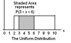
Figure 5.1: The graph shows a Uniform Distribution with the area between x=3 and x=6 shaded to repre-
sent the probability that the value of the random variable X is in the interval between 3 and 6.
Available for free at Connexions <http://cnx.org/content/col10522/1.40>
223
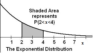
Figure 5.2: The graph shows an Exponential Distribution with the area between x=2 and x=4 shaded to
represent the probability that the value of the random variable X is in the interval between 2 and 4.
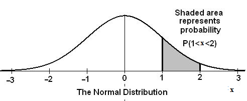
Figure 5.3: The graph shows the Standard Normal Distribution with the area between x=1 and x=2 shaded
to represent the probability that the value of the random variable X is in the interval between 1 and 2.
**With contributions from Roberta Bloom
5.2 Continuous Probability Functions2
We begin by defining a continuous probability density function. We use the function notation f (x). Inter-
mediate algebra may have been your first formal introduction to functions. In the study of probability, the
functions we study are special. We define the function f (x) so that the area between it and the x-axis is
equal to a probability. Since the maximum probability is one, the maximum area is also one.
For continuous probability distributions, PROBABILITY = AREA.
2This content is available online at <http://cnx.org/content/m16805/1.9/>.
Available for free at Connexions <http://cnx.org/content/col10522/1.40>
224
CHAPTER 5. CONTINUOUS RANDOM VARIABLES
Example 5.1
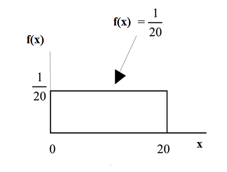
Consider the function f (x) = 1 for 0 ≤ x ≤ 20. x = a real number. The graph of f (x) = 1 is a
20
20
horizontal line. However, since 0 ≤ x ≤ 20 , f (x) is restricted to the portion between x = 0 and
x = 20, inclusive .
f (x) = 1 for 0 ≤ x ≤ 20.
20
The graph of f (x) = 1 is a horizontal line segment when 0 ≤ x ≤ 20.
20
The area between f (x) = 1 where 0 ≤ x ≤ 20 and the x-axis is the area of a rectangle with base
20
= 20 and height = 1 .
20
AREA = 20 · 1 = 1
20
This particular function, where we have restricted x so that the area between the function and
the x-axis is 1, is an example of a continuous probability density function. It is used as a tool to
calculate probabilities.
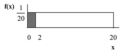
Suppose we want to find the area between f (x) = 1 and the x-axis where 0 < x < 2 .
20
AREA = (2 − 0) · 1 = 0.1
20
(2 − 0) = 2 = base of a rectangle
1 = the height.
20
The area corresponds to a probability. The probability that x is between 0 and 2 is 0.1, which can
be written mathematically as P(0<x<2) = P(x<2) = 0.1.
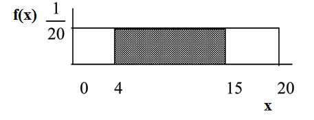
Suppose we want to find the area between f (x) = 1 and the x-axis where 4 < x < 15 .
20
Available for free at Connexions <http://cnx.org/content/col10522/1.40>
225
AREA = (15 − 4) · 1 = 0.55
20
(15 − 4) = 11 = the base of a rectangle
1 = the height.
20
The area corresponds to the probability P (4 < x < 15) = 0.55.
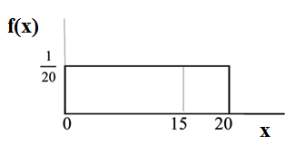
Suppose we want to find P (x = 15). On an x-y graph, x = 15 is a vertical line. A vertical line has
no width (or 0 width). Therefore, P (x = 15) = (base)(height) = (0)
1
= 0.
20
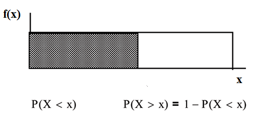
P (X ≤ x) (can be written as P (X < x) for continuous distributions) is called the cumulative dis-
tribution function or CDF. Notice the "less than or equal to" symbol. We can use the CDF to
calculate P (X > x) . The CDF gives "area to the left" and P (X > x) gives "area to the right." We
calculate P (X > x) for continuous distributions as follows: P (X > x) = 1 − P (X < x).
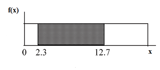
Label the graph with f (x) and x. Scale the x and y axes with the maximum x and y values.
f (x) = 1 , 0 ≤ x ≤ 20.
20
P (2.3 < x < 12.7) = (base) (height) = (12.7 − 2.3)
1
= 0.52
20
Available for free at Connexions <http://cnx.org/content/col10522/1.40>
226
CHAPTER 5. CONTINUOUS RANDOM VARIABLES
5.3 The Uniform Distribution3
Example 5.2
The previous problem is an example of the uniform probability distribution.
Illustrate the uniform distribution. The data that follows are 55 smiling times, in seconds, of an
eight-week old baby.
10.4
19.6
18.8
13.9
17.8
16.8
21.6
17.9
12.5
11.1
4.9
12.8
14.8
22.8
20.0
15.9
16.3
13.4
17.1
14.5
19.0
22.8
1.3
0.7
8.9
11.9
10.9
7.3
5.9
3.7
17.9
19.2
9.8
5.8
6.9
2.6
5.8
21.7
11.8
3.4
2.1
4.5
6.3
10.7
8.9
9.4
9.4
7.6
10.0
3.3
6.7
7.8
11.6
13.8
18.6
Table 5.1
sample mean = 11.49 and sample standard deviation = 6.23
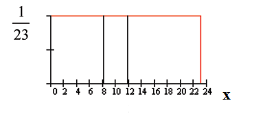
We will assume that the smiling times, in seconds, follow a uniform distribution between 0 and 23
seconds, inclusive. This means that any smiling time from 0 to and including 23 seconds is equally
likely. The histogram that could be constructed from the sample is an empirical distribution that
closely matches the theoretical uniform distribution.
Let X = length, in seconds, of an eight-week old baby’s smile.
The notation for the uniform distribution is
X ∼ U (a,b) where a = the lowest value of x and b = the highest value of x.
The probability density function is f (x) = 1 for a ≤ x ≤ b.
b−a
For this example, x ∼ U (0, 23) and f (x) =
1
for 0 ≤ x ≤ 23.
23−0
Formulas for the theoretical mean and standard deviation are
µ = a+b and
2
σ =
(b−a)2
12
For this problem, the theoretical mean and standard deviation are
µ = 0+23 = 11.50 seconds and
= 6.64 seconds
2
σ =
(23−0)2
12
Notice that the theoretical mean and standard deviation are close to the sample mean and standard
deviation.
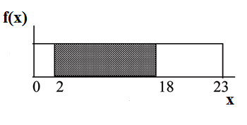
Example 5.3
Problem 1
What is the probability that a randomly chosen eight-week old baby smiles between 2 and 18
seconds?
Solution
Find P (2 < x < 18).
3This content is available online at <http://cnx.org/content/m16819/1.17/>.
Available for free at Connexions <http://cnx.org/content/col10522/1.40>
227
P (2 < x < 18) = (base) (height) = (18 − 2) · 1 = 16 .
23
23
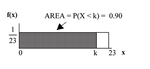
Problem 2
Find the 90th percentile for an eight week old baby’s smiling time.
Solution
Ninety percent of the smiling times fall below the 90th percentile, k, so P (x < k) = 0.90
P (x < k) = 0.90
(base) (height) = 0.90
(k − 0) · 1 = 0.90
23
k = 23 · 0.90 = 20.7
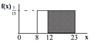
Problem 3
Find the probability that a random eight week old baby smiles more than 12 seconds KNOWING
that the baby smiles MORE THAN 8 SECONDS.
Solution
Find P (x > 12|x > 8) There are two ways to do the problem. For the first way, use the fact that
this is a conditional and changes the sample space. The graph illustrates the new sample space.
You already know the baby smiled more than 8 seconds.
Write a new f (x): f (x) =
1
= 1
23−8
15
for 8 < x < 23
P (x > 12|x > 8) = (23 − 12) · 1 = 11
15
15
Available for free at Connexions <http://cnx.org/content/col10522/1.40>
228
CHAPTER 5. CONTINUOUS RANDOM VARIABLES
For the second way, use the conditional formula from Probability Topics with the original distri-
bution X ∼ U (0, 23):
P (A|B) = P(A AND B) For this problem, A is (x > 12) and B is (x > 8).
P(B)
11
So, P (x > 12|x > 8) = (x>12 AND x>8) = P(x>12) = 23 = 0.733
P(x>8)
P(x>8)
15
23
Example 5.4
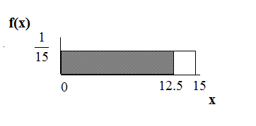
Uniform: The amount of time, in minutes, that a person must wait for a bus is uniformly dis-
tributed between 0 and 15 minutes, inclusive.
Problem 1
What is the probability that a person waits fewer than 12.5 minutes?
Solution
Let X = the number of minutes a person must wait for a bus. a = 0 and b = 15. x ∼ U (0, 15). Write
the probability density function. f (x) =
1
= 1 for 0 ≤ x ≤ 15.
15−0
15
Find P (x < 12.5). Draw a graph.
P (x < k) = (base) (height) = (12.5 − 0) · 1 = 0.8333
15
The probability a person waits less than 12.5 minutes is 0.8333.
Available for free at Connexions <http://cnx.org/content/col10522/1.40>
229
Problem 2
On the average, how long must a person wait?
Find the mean, µ, and the standard deviation, σ.
Solution
µ = a+b = 15+0 = 7.5. On the average, a person must wait 7.5 minutes.
2
2
σ =
(b−a)2 =
(15−0)2 = 4.3. The Standard deviation is 4.3 minutes.
12
12
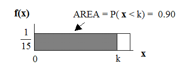
Problem 3
Ninety percent of the time, the time a person must wait falls below what value?
NOTE: This asks for the 90th percentile.
Solution
Find the 90th percentile. Draw a graph. Let k = the 90th percentile.
P (x < k) = (base) (height) = (k − 0) ·
1
15
0.90 = k · 1
15
k = (0.90) (15) = 13.5
k is sometimes called a critical value.
The 90th percentile is 13.5 minutes. Ninety percent of the time, a person must wait at most 13.5
minutes.
Example 5.5
Uniform: Suppose the time it takes a nine-year old to eat a donut is between 0.5 and 4 minutes,
inclusive. Let X = the time, in minutes, it takes a nine-year old child to eat a donut. Then X ∼
U (0.5, 4).
Problem 1
(Solution on p. 257.)
The probability that a randomly selected nine-year old child eats a donut in at least two minutes
is _______.
Problem 2
(Solution on p. 257.)
Find the probability that a different nine-year old child eats a donut in more than 2 minutes given
that the child has already been eating the donut for more than 1.5 minutes.
Available for free at Connexions <http://cnx.org/content/col10522/1.40>
230
CHAPTER 5. CONTINUOUS RANDOM VARIABLES
The second probability question has a conditional (refer to "Probability Topics (Section 3.1)"). You
are asked to find the probability that a nine-year old child eats a donut in more than 2 minutes
given that the child has already been eating the donut for more than 1.5 minutes. Solve the prob-
lem two different ways (see the first example (Example 5.2)). You must reduce the sample space.
First way: Since you already know the child has already been eating the donut for more than 1.5
minutes, you are no longer starting at a = 0.5 minutes. Your starting point is 1.5 minutes.
Write a new f(x):
f (x) =
1
= 2
for 1.5 ≤ x ≤ 4.
4−1.5
5
Find P (x > 2|x > 1.5). Draw a graph.
P (x > 2|x > 1.5) = (base) (new height) = (4 − 2) (2/5) =?
The probability that a nine-year old child eats a donut in more than 2 minutes given that the child
has already been eating the donut for more than 1.5 minutes is 4 .
5
Second way: Draw the original graph for x ∼ U (0.5, 4). Use the conditional formula
2
P (x > 2|x > 1.5) = P(x>2 AND x>1.5) = P(x>2) = 3.5 = 0.8 = 4
P(x>1.5)
P(x>1.5)
2.5
5
3.5
NOTE: See "Summary of the Uniform and Exponential Probability Distributions (Section 5.5)" for
a full summary.
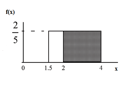
Example 5.6
Uniform: Ace Heating and Air Conditioning Service finds that the amount of time a repairman
needs to fix a furnace is uniformly distributed between 1.5 and 4 hours. Let x = the time needed
to fix a furnace. Then x ∼ U (1.5, 4).
1. Find the problem that a randomly selected furnace repair requires more than 2 hours.
2. Find the probability that a randomly selected furnace repair requires less than 3 hours.
3. Find the 30th percentile of furnace repair times.
4. The longest 25% of repair furnace repairs take at least how long? (In other words: Find the
minimum time for the longest 25% of repair times.) What percentile does this represent?
5. Find the mean and standard deviation
Problem 1
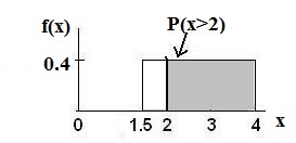
Find the probability that a randomly selected furnace repair requires longer than 2 hours.
Solution
To find f (x): f (x) =
1
= 1 so f (x) = 0.4
4−1.5
2.5
Available for free at Connexions <http://cnx.org/content/col10522/1.40>
231
P(x>2) = (base)(height) = (4 − 2)(0.4) = 0.8
Example 4 Figure 1
Figure 5.4: Uniform Distribution between 1.5 and 4 with shaded area between 2 and 4 representing the
probability that the repair time x is greater than 2
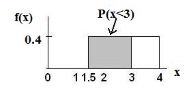
Problem 2
Find the probability that a randomly selected furnace repair requires less than 3 hours. Describe
how the graph differs from the graph in the first part of this example.
Solution
P (x < 3) = (base)(height) = (3 − 1.5)(0.4) = 0.6
The graph of the rectangle showing the entire distribution would remain the same. However the
graph should be shaded between x=1.5 and x=3. Note that the shaded area starts at x=1.5 rather
than at x=0; since X∼U(1.5,4), x can not be less than 1.5.
Example 4 Figure 2
Figure 5.5: Uniform Distribution between 1.5 and 4 with shaded area between 1.5 and 3 representing the
probability that the repair time x is less than 3
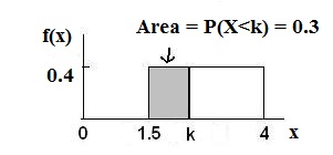
Problem 3
Find the 30th percentile of furnace repair times.
Solution
Available for free at Connexions <http://cnx.org/content/col10522/1.40>
232
CHAPTER 5. CONTINUOUS RANDOM VARIABLES
Example 4 Figure 3
Figure 5.6: Uniform Distribution between 1.5 and 4 with an area of 0.30 shaded to the left, representing the
shortest 30% of repair times.
P (x < k) = 0.30
P (x < k) = (base) (height) = (k − 1.5) · (0.4)
0.3 = (k − 1.5) (0.4) ; Solve to find k:
0.75 = k − 1.5 , obtained by dividing both sides by 0.4
k = 2.25 , obtained by adding 1.5 to both sides
The 30th percentile of repair times is 2.25 hours. 30% of repair times are 2.5 hours or less.
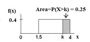
Problem 4
The longest 25% of furnace repair times take at least how long? (Find the minimum time for
the longest 25% of repairs.)
Solution
Example 4 Figure 4
Figure 5.7: Uniform Distribution between 1.5 and 4 with an area of 0.25 shaded to the right representing
the longest 25% of repair times.
P (x > k) = 0.25
P (x > k) = (base) (height) = (4 − k) · (0.4)
0.25 = (4 − k)(0.4) ; Solve for k:
Available for free at Connexions <http://cnx.org/content/col10522/1.40>
233
0.625 = 4 − k , obtained by dividing both sides by 0.4
−3.375 = −k , obtained by subtracting 4 from both sides
k=3.375
The longest 25% of furnace repairs take at least 3.375 hours (3.375 hours or longer).
Note: Since 25% of repair times are 3.375 hours or longer, that means that 75% of repair times are
3.375 hours or less. 3.375 hours is the 75th percentile of furnace repair times.
Problem 5
Find the mean and standard deviation
Solution
µ = a+b and
2
σ =
(b−a)2
12