CHAPTER 2. DESCRIPTIVE STATISTICS
in the town you want to move to. In this town, can you afford 34% of the houses or 66% of the
houses?
**With contributions from Roberta Bloom
2.7 Measures of the Center of the Data10
The "center" of a data set is also a way of describing location. The two most widely used measures of the
"center" of the data are the mean (average) and the median. To calculate the mean weight of 50 people,
add the 50 weights together and divide by 50. To find the median weight of the 50 people, order the data
and find the number that splits the data into two equal parts (previously discussed under box plots in this
chapter). The median is generally a better measure of the center when there are extreme values or outliers
because it is not affected by the precise numerical values of the outliers. The mean is the most common
measure of the center.
NOTE: The words "mean" and "average" are often used interchangeably. The substitution of one
word for the other is common practice. The technical term is "arithmetic mean" and "average" is
technically a center location. However, in practice among non-statisticians, "average" is commonly
accepted for "arithmetic mean."
The mean can also be calculated by multiplying each distinct value by its frequency and then dividing the
sum by the total number of data values. The letter used to represent the sample mean is an x with a bar
over it (pronounced "x bar"): x.
The Greek letter µ (pronounced "mew") represents the population mean. One of the requirements for the
sample mean to be a good estimate of the population mean is for the sample taken to be truly random.
To see that both ways of calculating the mean are the same, consider the sample:
1; 1; 1; 2; 2; 3; 4; 4; 4; 4; 4
1 + 1 + 1 + 2 + 2 + 3 + 4 + 4 + 4 + 4 + 4
x =
= 2.7
(2.6)
11
3 × 1 + 2 × 2 + 1 × 3 + 5 × 4
x =
= 2.7
(2.7)
11
In the second calculation for the sample mean, the frequencies are 3, 2, 1, and 5.
You can quickly find the location of the median by using the expression n+1 .
2
The letter n is the total number of data values in the sample. If n is an odd number, the median is the middle
value of the ordered data (ordered smallest to largest). If n is an even number, the median is equal to the
two middle values added together and divided by 2 after the data has been ordered. For example, if the
total number of data values is 97, then n+1 = 97+1 = 49. The median is the 49th value in the ordered data.
2
2
If the total number of data values is 100, then n+1 = 100+1 = 50.5. The median occurs midway between the
2
2
50th and 51st values. The location of the median and the value of the median are not the same. The upper
case letter M is often used to represent the median. The next example illustrates the location of the median
and the value of the median.
Example 2.17
AIDS data indicating the number of months an AIDS patient lives after taking a new antibody
drug are as follows (smallest to largest):
10This content is available online at <http://cnx.org/content/m17102/1.13/>.
Available for free at Connexions <http://cnx.org/content/col10522/1.40>
77
3; 4; 8; 8; 10; 11; 12; 13; 14; 15; 15; 16; 16; 17; 17; 18; 21; 22; 22; 24; 24; 25; 26; 26; 27; 27; 29; 29; 31; 32;
33; 33; 34; 34; 35; 37; 40; 44; 44; 47
Calculate the mean and the median.
Solution
The calculation for the mean is:
x = [3+4+(8)(2)+10+11+12+13+14+(15)(2)+(16)(2)+...+35+37+40+(44)(2)+47] = 23.6
40
To find the median, M, first use the formula for the location. The location is:
n+1 = 40+1 = 20.5
2
2
Starting at the smallest value, the median is located between the 20th and 21st values (the two
24s):
3; 4; 8; 8; 10; 11; 12; 13; 14; 15; 15; 16; 16; 17; 17; 18; 21; 22; 22; 24; 24; 25; 26; 26; 27; 27; 29; 29; 31; 32;
33; 33; 34; 34; 35; 37; 40; 44; 44; 47
M = 24+24 = 24
2
The median is 24.
Using the TI-83,83+,84, 84+ Calculators
Calculator Instructions are located in the menu item 14:Appendix (Notes for the TI-83, 83+, 84,
84+ Calculators).
• Enter data into the list editor. Press STAT 1:EDIT
• Put the data values in list L1.
• Press STAT and arrow to CALC. Press 1:1-VarStats. Press 2nd 1 for L1 and ENTER.
• Press the down and up arrow keys to scroll.
x = 23.6, M = 24
Example 2.18
Suppose that, in a small town of 50 people, one person earns $5,000,000 per year and the other 49
each earn $30,000. Which is the better measure of the "center," the mean or the median?
Solution
x = 5000000+49×30000 = 129400
50
M = 30000
(There are 49 people who earn $30,000 and one person who earns $5,000,000.)
The median is a better measure of the "center" than the mean because 49 of the values are 30,000
and one is 5,000,000. The 5,000,000 is an outlier. The 30,000 gives us a better sense of the middle of
the data.
Another measure of the center is the mode. The mode is the most frequent value. If a data set has two
values that occur the same number of times, then the set is bimodal.
Example 2.19: Statistics exam scores for 20 students are as follows
Statistics exam scores for 20 students are as follows:
Available for free at Connexions <http://cnx.org/content/col10522/1.40>
78
CHAPTER 2. DESCRIPTIVE STATISTICS
50 ; 53 ; 59 ; 59 ; 63 ; 63 ; 72 ; 72 ; 72 ; 72 ; 72 ; 76 ; 78 ; 81 ; 83 ; 84 ; 84 ; 84 ; 90 ; 93
Problem
Find the mode.
Solution
The most frequent score is 72, which occurs five times. Mode = 72.
Example 2.20
Five real estate exam scores are 430, 430, 480, 480, 495. The data set is bimodal because the scores
430 and 480 each occur twice.
When is the mode the best measure of the "center"? Consider a weight loss program that advertises
a mean weight loss of six pounds the first week of the program. The mode might indicate that most
people lose two pounds the first week, making the program less appealing.
NOTE: The mode can be calculated for qualitative data as well as for quantitative data.
Statistical software will easily calculate the mean, the median, and the mode. Some graphing
calculators can also make these calculations. In the real world, people make these calculations
using software.
2.7.1 The Law of Large Numbers and the Mean
The Law of Large Numbers says that if you take samples of larger and larger size from any population,
then the mean x of the sample is very likely to get closer and closer to µ. This is discussed in more detail in
The Central Limit Theorem.
NOTE: The formula for the mean is located in the Summary of Formulas (Section 2.10) section
course.
2.7.2 Sampling Distributions and Statistic of a Sampling Distribution
You can think of a sampling distribution as a relative frequency distribution with a great many samples.
(See Sampling and Data for a review of relative frequency). Suppose thirty randomly selected students
were asked the number of movies they watched the previous week. The results are in the relative frequency
table shown below.
# of movies
Relative Frequency
0
5/30
1
15/30
2
6/30
3
4/30
4
1/30
Table 2.6
Available for free at Connexions <http://cnx.org/content/col10522/1.40>
79
If you let the number of samples get very large (say, 300 million or more), the relative frequency table
becomes a relative frequency distribution.
A statistic is a number calculated from a sample. Statistic examples include the mean, the median and the
mode as well as others. The sample mean x is an example of a statistic which estimates the population
mean µ.
2.8 Skewness and the Mean, Median, and Mode11
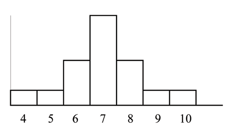
Consider the following data set:
4 ; 5 ; 6 ; 6 ; 6 ; 7 ; 7 ; 7 ; 7 ; 7 ; 7 ; 8 ; 8 ; 8 ; 9 ; 10
This data set produces the histogram shown below. Each interval has width one and each value is located
in the middle of an interval.
The histogram displays a symmetrical distribution of data. A distribution is symmetrical if a vertical line
can be drawn at some point in the histogram such that the shape to the left and the right of the vertical
line are mirror images of each other. The mean, the median, and the mode are each 7 for these data. In a
perfectly symmetrical distribution, the mean and the median are the same. This example has one mode
(unimodal) and the mode is the same as the mean and median. In a symmetrical distribution that has two
modes (bimodal), the two modes would be different from the mean and median.
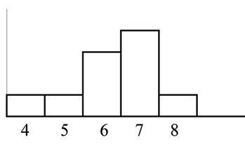
The histogram for the data:
4 ; 5 ; 6 ; 6 ; 6 ; 7 ; 7 ; 7 ; 7 ; 8
is not symmetrical. The right-hand side seems "chopped off" compared to the left side. The shape distribu-
tion is called skewed to the left because it is pulled out to the left.
11This content is available online at <http://cnx.org/content/m17104/1.9/>.
Available for free at Connexions <http://cnx.org/content/col10522/1.40>
80
CHAPTER 2. DESCRIPTIVE STATISTICS
The mean is 6.3, the median is 6.5, and the mode is 7. Notice that the mean is less than the median and
they are both less than the mode. The mean and the median both reflect the skewing but the mean more
so.
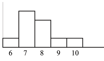
The histogram for the data:
6 ; 7 ; 7 ; 7 ; 7 ; 8 ; 8 ; 8 ; 9 ; 10
is also not symmetrical. It is skewed to the right.
The mean is 7.7, the median is 7.5, and the mode is 7. Of the three statistics, the mean is the largest, while
the mode is the smallest. Again, the mean reflects the skewing the most.
To summarize, generally if the distribution of data is skewed to the left, the mean is less than the median,
which is often less than the mode. If the distribution of data is skewed to the right, the mode is often less
than the median, which is less than the mean.
Skewness and symmetry become important when we discuss probability distributions in later chapters.
Available for free at Connexions <http://cnx.org/content/col10522/1.40>
81
2.9 Measures of the Spread of the Data12
An important characteristic of any set of data is the variation in the data. In some data sets, the data values
are concentrated closely near the mean; in other data sets, the data values are more widely spread out from
the mean. The most common measure of variation, or spread, is the standard deviation.
The standard deviation is a number that measures how far data values are from their mean.
The standard deviation
• provides a numerical measure of the overall amount of variation in a data set
• can be used to determine whether a particular data value is close to or far from the mean
The standard deviation provides a measure of the overall variation in a data set
The standard deviation is always positive or 0. The standard deviation is small when the data are all
concentrated close to the mean, exhibiting little variation or spread. The standard deviation is larger when
the data values are more spread out from the mean, exhibiting more variation.
Suppose that we are studying waiting times at the checkout line for customers at supermarket A and
supermarket B; the average wait time at both markets is 5 minutes. At market A, the standard deviation
for the waiting time is 2 minutes; at market B the standard deviation for the waiting time is 4 minutes.
Because market B has a higher standard deviation, we know that there is more variation in the wait-
ing times at market B. Overall, wait times at market B are more spread out from the average; wait times at
market A are more concentrated near the average.
The standard deviation can be used to determine whether a data value is close to or far from the mean.
Suppose that Rosa and Binh both shop at Market A. Rosa waits for 7 minutes and Binh waits for 1 minute
at the checkout counter. At market A, the mean wait time is 5 minutes and the standard deviation is 2
minutes. The standard deviation can be used to determine whether a data value is close to or far from the
mean.
Rosa waits for 7 minutes:
• 7 is 2 minutes longer than the average of 5; 2 minutes is equal to one standard deviation.
• Rosa’s wait time of 7 minutes is 2 minutes longer than the average of 5 minutes.
• Rosa’s wait time of 7 minutes is one standard deviation above the average of 5 minutes.
Binh waits for 1 minute.
• 1 is 4 minutes less than the average of 5; 4 minutes is equal to two standard deviations.
• Binh’s wait time of 1 minute is 4 minutes less than the average of 5 minutes.
• Binh’s wait time of 1 minute is two standard deviations below the average of 5 minutes.
• A data value that is two standard deviations from the average is just on the borderline for what many
statisticians would consider to be far from the average. Considering data to be far from the mean if it
is more than 2 standard deviations away is more of an approximate "rule of thumb" than a rigid rule.
In general, the shape of the distribution of the data affects how much of the data is further away than
2 standard deviations. (We will learn more about this in later chapters.)
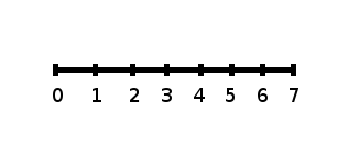
The number line may help you understand standard deviation. If we were to put 5 and 7 on a number line,
7 is to the right of 5. We say, then, that 7 is one standard deviation to the right of 5 because
5 + (1) (2) = 7.
12This content is available online at <http://cnx.org/content/m17103/1.15/>.
Available for free at Connexions <http://cnx.org/content/col10522/1.40>
82
CHAPTER 2. DESCRIPTIVE STATISTICS
If 1 were also part of the data set, then 1 is two standard deviations to the left of 5 because
5 + (−2) (2) = 1.
• In general, a value = mean + (#ofSTDEV)(standard deviation)
• where #ofSTDEVs = the number of standard deviations
• 7 is one standard deviation more than the mean of 5 because: 7=5+(1)(2)
• 1 is two standard deviations less than the mean of 5 because: 1=5+(−2)(2)
The equation value = mean + (#ofSTDEVs)(standard deviation) can be expressed for a sample and for a
population:
• sample: x = x + (#o f STDEV) (s)
• Population: x = µ + (#o f STDEV) ( σ)
The lower case letter s represents the sample standard deviation and the Greek letter σ (sigma, lower case)
represents the population standard deviation.
The symbol x is the sample mean and the Greek symbol µ is the population mean.
Calculating the Standard Deviation
If x is a number, then the difference "x - mean" is called its deviation. In a data set, there are as many
deviations as there are items in the data set. The deviations are used to calculate the standard deviation.
If the numbers belong to a population, in symbols a deviation is x − µ . For sample data, in symbols a
deviation is x− x .
The procedure to calculate the standard deviation depends on whether the numbers are the entire popula-
tion or are data from a sample. The calculations are similar, but not identical. Therefore the symbol used
to represent the standard deviation depends on whether it is calculated from a population or a sample.
The lower case letter s represents the sample standard deviation and the Greek letter σ (sigma, lower case)
represents the population standard deviation. If the sample has the same characteristics as the population,
then s should be a good estimate of σ.
To calculate the standard deviation, we need to calculate the variance first. The variance is an average of
the squares of the deviations (the x− x values for a sample, or the x − µ values for a population). The
symbol 2
σ
represents the population variance; the population standard deviation σ is the square root of
the population variance. The symbol s2 represents the sample variance; the sample standard deviation s is
the square root of the sample variance. You can think of the standard deviation as a special average of the
deviations.
If the numbers come from a census of the entire population and not a sample, when we calculate the aver-
age of the squared deviations to find the variance, we divide by N, the number of items in the population.
If the data are from a sample rather than a population, when we calculate the average of the squared devi-
ations, we divide by n-1, one less than the number of items in the sample. You can see that in the formulas
below.
Available for free at Connexions <http://cnx.org/content/col10522/1.40>
83
Formulas for the Sample Standard Deviation
•
Σ
Σ
s =
(x−x)2 or s =
f ·(x−x)2
n−1
n−1
• For the sample standard deviation, the denominator is n-1, that is the sample size MINUS 1.
Formulas for the Population Standard Deviation
•
Σ(x− µ)2
Σ f ·(x− µ)2
σ =
or
N
σ =
N
• For the population standard deviation, the denominator is N, the number of items in the population.
In these formulas, f represents the frequency with which a value appears. For example, if a value appears
once, f is 1. If a value appears three times in the data set or population, f is 3.
Sampling Variability of a Statistic
The statistic of a sampling distribution was discussed in Descriptive Statistics: Measuring the Center of
the Data. How much the statistic varies from one sample to another is known as the sampling variability of
a statistic. You typically measure the sampling variability of a statistic by its standard error. The standard
error of the mean is an example of a standard error. It is a special standard deviation and is known as the
standard deviation of the sampling distribution of the mean. You will cover the standard error of the mean
in The Central Limit Theorem (not now). The notation for the standard error of the mean is σ
√
where σ is
n
the standard deviation of the population and n is the size of the sample.
NOTE:
In practice, USE A CALCULATOR OR COMPUTER SOFTWARE TO CALCULATE
THE STANDARD DEVIATION. If you are using a TI-83,83+,84+ calculator, you need to select
the appropriate standard deviation σ x or sx from the summary statistics. We will concentrate on
using and interpreting the information that the standard deviation gives us. However you should
study the following step-by-step example to help you understand how the standard deviation
measures variation from the mean.
Example 2.21
In a fifth grade class, the teacher was interested in the average age and the sample standard
deviation of the ages of her students. The following data are the ages for a SAMPLE of n = 20 fifth
grade students. The ages are rounded to the nearest half year:
9 ; 9.5 ; 9.5 ; 10 ; 10 ; 10 ; 10 ; 10.5 ; 10.5 ; 10.5 ; 10.5 ; 11 ; 11 ; 11 ; 11 ; 11 ; 11 ; 11.5 ; 11.5 ; 11.5
9 + 9.5 × 2 + 10 × 4 + 10.5 × 4 + 11 × 6 + 11.5 × 3
x =
= 10.525
(2.8)
20
The average age is 10.53 years, rounded to 2 places.
The variance may be calculated by using a table. Then the standard deviation is calculated by
taking the square root of the variance. We will explain the parts of the table after calculating s.
Data
Freq.
Deviations
Deviations2
(Freq.)(Deviations2)
x
f
(x − x)
(x − x)2
( f ) (x − x)2
9
1
9 − 10.525 = −1.525
(−1.525)2 = 2.325625
1 × 2.325625 = 2.325625
9.5
2
9.5 − 10.525 = −1.025
(−1.025)2 = 1.050625
2 × 1.050625 = 2.101250
10
4
10 − 10.525 = −0.525
(−0.525)2 = 0.275625
4 × .275625 = 1.1025
10.5
4
10.5 − 10.525 = −0.025
(−0.025)2 = 0.000625
4 × .000625 = .0025
11
6
11 − 10.525 = 0.475
(0.475)2 = 0.225625
6 × .225625 = 1.35375
11.5
3
11.5 − 10.525 = 0.975
(0.975)2 = 0.950625
3 × .950625 = 2.851875
Available for free at Connexions <http://cnx.org/content/col10522/1.40>
84
CHAPTER 2. DESCRIPTIVE STATISTICS
Table 2.7
The sample variance, s2, is equal to the sum of the last column (9.7375) divided by the total number
of data values minus one (20 - 1):
s2 = 9.7375 = 0.5125
20−1
The sample standard deviation s is equal to the square root of the sample variance:
√
s =
0.5125 = .0715891 Rounded to two decimal places, s = 0.72
Typically, you do the calculation for the standard deviation on your calculator or computer. The
intermediate results are not rounded. This is done for accuracy.
Problem 1
Verify the mean and standard deviation calculated above on your calculator or computer.
Solution
Using the TI-83,83+,84+ Calculators
• Enter data into the list editor. Press STAT 1:EDIT. If necessary, clear the lists by arrowing up
into the name. Press CLEAR and arrow down.
• Put the data values (9, 9.5, 10, 10.5, 11, 11.5) into list L1 and the frequencies (1, 2, 4, 4, 6, 3)
into list L2. Use the arrow keys to move around.
• Press STAT and arrow to CALC. Press 1:1-VarStats and enter L1 (2nd 1), L2 (2nd 2). Do not
forget