DSPA by Douglas Jones, Don Johnson, et al - HTML preview

/ Home / Mathematics (Academic) / DSPA

PLEASE NOTE: This is an HTML preview only and some elements such as links or page numbers may be incorrect.
Download the book in PDF, ePub for a complete version.

variance is

Note that in general, each Hi( w) , and thus the variance at the

output due to each quantizer, is different; for example, the system as seen by a quantizer at the

input to the first delay state in the Direct-Form II IIR filter structure to the output, call it n 4 , is

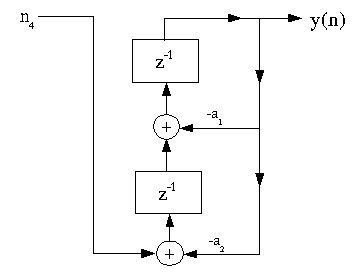
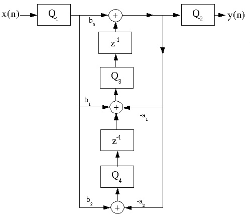
Figure 6.28.

with a transfer function

which can be evaluated at z= ⅇⅈw to obtain the frequency

response.

A general approach to find Hi( w) is to write state equations for the equivalent structure as seen by

ni , and to determine the transfer function according to H( z)= C( zI− A)-1 B+ d .

Figure 6.29.

Exercise 5.

The above figure illustrates the quantization points in a typical implementation of a Direct-Form

II IIR second-order section. What is the total variance of the output error due to all of the

quantizers in the system?

By making the assumption that each Qi represents a noise source that is white, independent of the

other sources, and additive,

Figure 6.30.

the variance at the output is the sum of the variances at the output due to each noise source:

The variance due to each noise source at the output can be determined from

; note that S

n ( w)= σ

by our assumptions, and H

i( w) is the transfer function

from the noise source to the output.

IIR Coefficient Quantization Analysis*

Coefficient quantization is an important concern with IIR filters, since straigthforward

quantization often yields poor results, and because quantization can produce unstable filters.

Sensitivity analysis

The performance and stability of an IIR filter depends on the pole locations, so it is important to

know how quantization of the filter coefficients ak affects the pole locations pj . The denominator

polynomial is

We wish to know

, which, for small deviations,

will tell us that a δ change in ak yields an

change in the pole location.

is the

sensitivity of the pole location to quantization of ak . We can find

using the chain rule.

⇓

which is

()

Note that as the poles get closer together, the sensitivity increases greatly. So as the filter order

increases and more poles get stuffed closer together inside the unit circle, the error introduced by

coefficient quantization in the pole locations grows rapidly.

How can we reduce this high sensitivity to IIR filter coefficient quantization?

Solution

Cascade or parallel form implementations! The numerator and denominator polynomials can be factored off-line at very high precision and grouped into second-order sections, which are then

quantized section by section. The sensitivity of the quantization is thus that of second-order,

rather than N-th order, polynomials. This yields major improvements in the frequency response of

the overall filter, and is almost always done in practice.

Note that the numerator polynomial faces the same sensitivity issues; the cascade form also

improves the sensitivity of the zeros, because they are also factored into second-order terms.

However, in the parallel form, the zeros are globally distributed across the sections, so they suffer

from quantization of all the blocks. Thus the cascade form preserves zero locations much better

than the parallel form, which typically means that the stopband behavior is better in the cascade

form, so it is most often used in practice.

Note on FIR Filters

On the basis of the preceding analysis, it would seem important to use cascade structures in

FIR filter implementations. However, most FIR filters are linear-phase and thus symmetric or

anti-symmetric. As long as the quantization is implemented such that the filter coefficients

retain symmetry, the filter retains linear phase. Furthermore, since all zeros off the unit circle

must appear in groups of four for symmetric linear-phase filters, zero pairs can leave the unit

circle only by joining with another pair. This requires relatively severe quantizations (enough

to completely remove or change the sign of a ripple in the amplitude response). This

"reluctance" of pole pairs to leave the unit circle tends to keep quantization from damaging

the frequency response as much as might be expected, enough so that cascade structures are

rarely used for FIR filters.

Exercise 6.

What is the worst-case pole pair in an IIR digital filter?

The pole pair closest to the real axis in the z-plane, since the complex-conjugate poles will be

closest together and thus have the highest sensitivity to quantization.

Quantized Pole Locations

In a direct-form or transpose-form implementation of a second-order section, the filter coefficients are quantized versions of the polynomial coefficients.

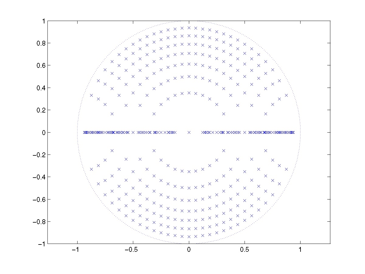
p= rⅇⅈθ D( z)= z 2−2 r cos( θ)+ r 2 So a 1=–(2 r cos( θ)) a 2= r 2 Thus the quantization of a 1 and a 2 to B bits restricts the radius r to

, and a 1=–(2Re( p))= kΔB The following figure

shows all stable pole locations after four-bit two's-complement quantization.

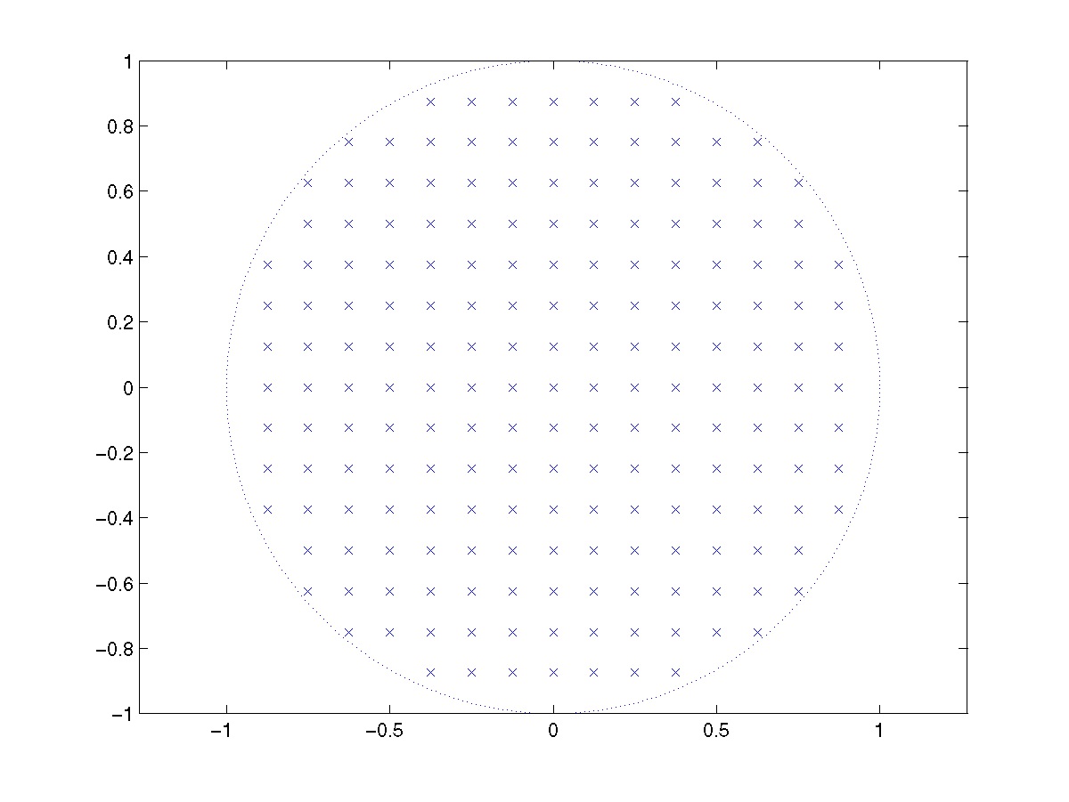
Figure 6.31.

Note the nonuniform distribution of possible pole locations. This might be good for poles near

r=1 ,

, but not so good for poles near the origin or the Nyquist frequency.

In the "normal-form" structures, a state-variable based realization, the poles are uniformly spaced.

Figure 6.32.

This can only be accomplished if the coefficients to be quantized equal the real and imaginary

parts of the pole location; that is, α 1= r cos( θ)=Re( r) α 2= r sin( θ)=Im( p) This is the case for a 2nd-order system with the state matrix

: The denominator polynomial is

()

Given any second-order filter coefficient set, we can write it as a state-space system, find a

transformation matrix T such that

is in normal form, and then implement the second-

order section using a structure corresponding to the state equations.

The normal form has a number of other advantages; both eigenvalues are equal, so it minimizes

the norm of Ax , which makes overflow less likely, and it minimizes the output variance due to

quantization of the state values. It is sometimes used when minimization of finite-precision

effects is critical.

Exercise 7.

What is the disadvantage of the normal form?

It requires more computation. The general state-variable equation requires nine multiplies,

rather than the five used by the Direct-Form II or Transpose-Form structures.

6.4. Overflow Problems and Solutions

Limit Cycles*

Large-scale limit cycles

When overflow occurs, even otherwise stable filters may get stuck in a large-scale limit cycle,

which is a short-period, almost full-scale persistent filter output caused by overflow.

Example 6.3.

Consider the second-order system

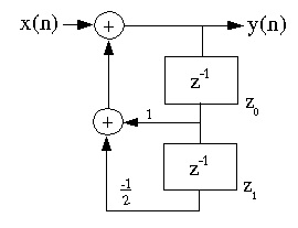
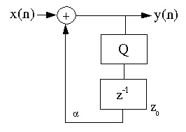
Figure 6.33.

with zero input and initial state values z 0[0]=0.8 , z 1[0]=-0.8 . Note y[ n]= z 0[ n+1] .

The filter is obviously stable, since the magnitude of the poles is

, which is well inside

the unit circle. However, with wraparound overflow, note that

, and

that

, so

even with zero input.

Clearly, such behavior is intolerable and must be prevented. Saturation arithmetic has been proved

to prevent zero-input limit cycles, which is one reason why all DSP microprocessors support this

feature. In many applications, this is considered sufficient protection. Scaling to prevent overflow

is another solution, if as well the inital state values are never initialized to limit-cycle-producing

values. The normal-form structure also reduces the chance of overflow.

Small-scale limit cycles

Small-scale limit cycles are caused by quantization. Consider the system

Figure 6.34.

Note that when

, rounding will quantize the output to the current level (with zero input),

so the output will remain at this level forever. Note that the maximum amplitude of this "small-

scale limit cycle" is achieved when

In a higher-order system, the

small-scale limit cycles are oscillatory in nature. Any quantization scheme that never increases

the magnitude of any quantized value prevents small-scale limit cycles.

Two's-complement truncation does not do this; it increases the magnitude of negative

numbers.

However, this introduces greater error and bias. Since the level of the limit cycles is proportional

to ΔB , they can be reduced by increasing the number of bits. Poles close to the unit circle increase

the magnitude and likelihood of small-scale limit cycles.

Scaling*

Overflow is clearly a serious problem, since the errors it introduces are very large. As we shall

see, it is also responsible for large-scale limit cycles, which cannot be tolerated. One way to

prevent overflow, or to render it acceptably unlikely, is to scale the input to a filter such that

overflow cannot (or is sufficiently unlikely to) occur.

Figure 6.35.

In a fixed-point system, the range of the input signal is limited by the fractional fixed-point

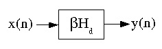
number representation to | x[ n]|≤1 . If we scale the input by multiplying it by a value β, 0< β<1 , then | βx[ n]|≤ β .

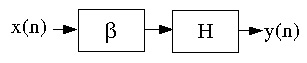
Another option is to incorporate the scaling directly into the filter coefficients.

Figure 6.36.

FIR Filter Scaling

What value of β is required so that the output of an FIR filter cannot overflow ( | y( n)|≤1 ,

| x( n)|≤1 )?

⇓

Alternatively, we can

incorporate the scaling directly into the filter, and require that

to prevent overflow.

IIR Filter Scaling

To prevent the output from overflowing in an IIR filter, the condition above still holds: ( M=∞ )

so an initial scaling factor

can be used, or the filter itself can be scaled.

However, it is also necessary to prevent the states from overflowing, and to prevent overflow at

any point in the signal flow graph where the arithmetic hardware would thereby produce errors. To

prevent the states from overflowing, we determine the transfer function from the input to all states

i, and scale the filter such that

Although this method of scaling guarantees no overflows, it is often too conservative. Note that a

worst-case signal is x( n)=sign( h(– n)) ; this input may be extremely unlikely. In the relatively

common situation in which the input is expected to be mainly a single-frequency sinusoid of

unknown frequency and amplitude less than 1, a scaling condition of | H( w)|≤1 is sufficient to

guarantee no overflow. This scaling condition is often used. If there are several potential overflow

locations i in the digital filter structure, the scaling conditions are | Hi( w)|≤1 where Hi( w) is the frequency response from the input to location i in the filter.

Even this condition may be excessively conservative, for example if the input is more-or-less

random, or if occasional overflow can be tolerated. In practice, experimentation and simulation

are often the best ways to optimize the scaling factors in a given application.

For filters implemented in the cascade form, rather than scaling for the entire filter at the

beginning, (which introduces lots of quantization of the input) the filter is usually scaled so that

each stage is just prevented from overflowing. This is best in terms of reducing the quantization

noise. The scaling factors are incorporated either into the previous or the next stage, whichever is

most convenient.

Some heurisitc rules for grouping poles and zeros in a cascade implementation are:

1. Order the poles in terms of decreasing radius. Take the pole pair closest to the unit circle and

group it with the zero pair closest to that pole pair (to minimize the gain in that section). Keep

doing this with all remaining poles and zeros.

2. Order the section with those with highest gain ( argmax| Hi( w)| ) in the middle, and those with

lower gain on the ends.

Leland B. Jackson [link] has an excellent intuitive discussion of finite-precision problems in digital filters. The book by Roberts and Mullis [link] is one of the most thorough in terms of detail.

References

1. Leland B. Jackson. (1989). Digital Filters and Signal Processing. (2nd Edition). Kluwer

Academic Publishers.

2. Richard A. Roberts and Clifford T. Mullis. (1987). Digital Signal Processing. Prentice Hall.

Glossary

Definition: State

the minimum additional information at time simplemath mathml-miitalicsn n, which, along with

all current and future input values, is necessary to compute all future outputs.

Solutions

Index

aliases, Impulse-Invariant Design

all-pass, Digital-to-Digital Frequency Transformations