()


()
So we have an all-digital formula for exact digital-to-digital rate changing!
3. Cost of computing sinc T′( mT 1− nT 0) : The solution is to precompute the table of sinc( t) values.
However, if
is not a rational fraction, an infinite number of samples will be needed, so
some approximation will have to be tolerated.
Rate transformation of any rate to any other rate can be accomplished digitally with
arbitrary precision (if some delay is acceptable). This method is used in practice in many
cases. We will examine a number of special cases and computational improvements, but in
some sense everything that follows are details; the above idea is the central idea in
multirate signal processing.
Useful references for the traditional material (everything except PRFBs) are Crochiere and
Rabiner, 1981 [link] and Crochiere and Rabiner, 1983 [link]. A more recent tutorial is Vaidyanathan [link]; see also Rioul and Vetterli [link]. References to most of the original papers can be found in these tutorials.
References
1. R.E. Crochiere and L.R. Rabiner. (1981, March). Interpolation and Decimation of Digital
Signals: A Tutorial Review. Proc. IEEE, 69(3), 300-331.
2. R.E. Crochiere and L.R. Rabiner. (1983). Multirate Digital Signal Processing. Englewood
Cliffs, NJ: Prentice-Hall.
3. P.P Vaidyanathan. (1990, January). Multirate Digital Filters, Filter Banks, Polyphase
Networks, and Applications: A Tutorial. Proc. IEEE, 78(1), 56-93.
4. O. Rioul and M. Vetterli. (1991, October). Wavelets and Signal Processing. IEEE Signal
Processing Magazine, 8(4), 14-38.
5.2. Interpolation, Decimation, and Rate Changing by


Integer Fractions*
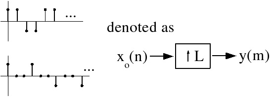
Interpolation: by an integer factor L
Interpolation means increasing the sampling rate, or filling in in-between samples. Equivalent to
sampling a bandlimited analog signal L times faster. For the ideal interpolator,
()
We wish to accomplish this digitally. Consider Equation and Figure 5.2.
()
Figure 5.2.
The DTFT of y( m) is
()
Since X 0( ω′) is periodic with a period of 2 π , X 0( Lω)= Y( ω) is periodic with a period of (see
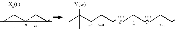

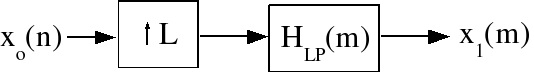
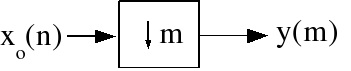
Figure 5.3.
By inserting zero samples between the samples of x 0( n) , we obtain a signal with a scaled
frequency response that simply replicates X 0( ω′) L times over a 2 π interval!
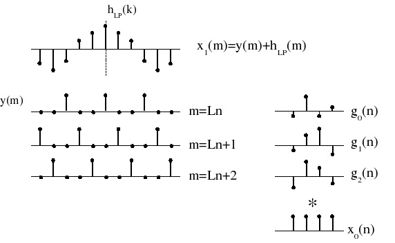
Obviously, the desired x 1( m) can be obtained simply by lowpass filtering y( m) to remove the
replicas.
()
x 1( m)= y( m)* hL( m)
Given
In practice, a finite-length lowpass filter is designed using any of the
methods studied so far (Figure 5.4).
Figure 5.4. Interpolator Block Diagram
Decimation: sampling rate reduction (by an integer factor M)
Let y( m)= x 0( Lm) (Figure 5.5)
Figure 5.5.
That is, keep only every L th sample (Figure 5.6)
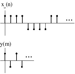


Figure 5.6.
In frequency (DTFT):
()
Now
for | ω|< π as shown in homework #1 , where X( k) is the
DFT of one period of the periodic sequence. In this case, X( k)=1 for k∈{0, 1, …, M−1} and
.
()
so
i.e. , we get digital aliasing.(Figure 5.7)
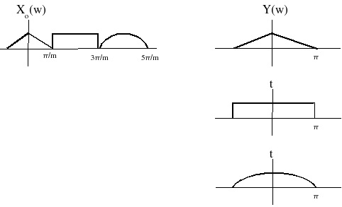

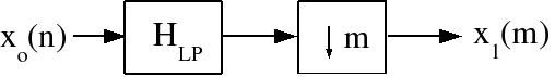


Figure 5.7.
Usually, we prefer not to have aliasing, so the downsampler is preceded by a lowpass filter to
remove all frequency components above
Figure 5.8.
Rate-Changing by a Rational Fraction L/M
This is easily accomplished by interpolating by a factor of L, then decimating by a factor of M
(Figure 5.9).
Figure 5.9.
The two lowpass filters can be combined into one LP filter with the lower cutoff,
Obviously, the computational complexity and simplicity of
implementation will depend on : 2/3 will be easier to implement than 1061/1060 !
5.3. Efficient Multirate Filter Structures*


Rate-changing appears expensive computationally, since for both decimation and interpolation the
lowpass filter is implemented at the higher rate. However, this is not necessary.
Interpolation
For the interpolator, most of the samples in the upsampled signal are zero, and thus require no
computation. (Figure 5.10)
Figure 5.10.
For
and p= m mod L ,
()
gp( n)= h( Ln+ p) Pictorially, this can be represented as in Figure 5.11.
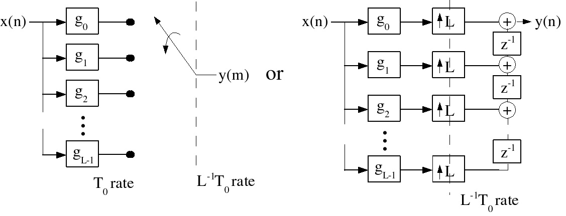


Figure 5.11.
These are called polyphase structures, and the gp( n) are called polyphase filters.
Computational cost
If h( m) is a length- N filter:
No simplification:
Polyphase structure:
where L is the number of filters, is the taps/filter,
and
is the rate.
Thus we save a factor of L by not being dumb.
For a given precision, N is proportional to L, (why?), so the computational cost does increase
with the interpolation rate.
Question
Can similar computational savings be obtained with IIR structures?
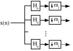
Efficient Decimation Structures

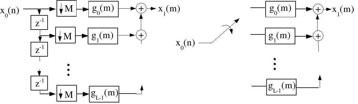

We only want every M th output, so we compute only the outputs of interest. (Figure 5.12)
Figure 5.12. Polyphase Decimation Structure
The decimation structures are flow-graph reversals of the interpolation structure. Although direct
implementation of the full filter for every M th sample is obvious and straightforward, these
polyphase structures give some idea as to how one might evenly partition the computation over M
cycles.
Efficient L/M rate changers
Interpolate by L and decimate by M (Figure 5.13).
Figure 5.13.
Combine the lowpass filters (Figure 5.14).
Figure 5.14.
We can couple the lowpass filter either to the interpolator or the decimator to implement it
efficiently (Figure 5.15).
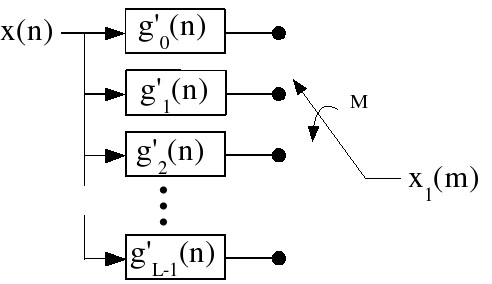


Figure 5.15.
Of course we only compute the polyphase filter output selected by the decimator.
Computational Cost
Every
, compute one polyphase filter of length , or
However,
note that N is proportional to max{ L, M} .
5.4. Filter Design for Multirate Systems*
The filter design techniques learned earlier can be applied to the design of filters in multirate systems, with a few twists.
Example 5.1.
Design a factor-of- L interpolator for use in a CD player, we might wish that the out-of-band
error be below the least significant bit, or 96dB down, and < 0.05 % error in the passband, so
these specifications could be used for optimal L∞ filter design.
In a CD player, the sampling rate is 44.1kHz, corresponding to a Nyquist frequency of 22.05kHz,
but the sampled signal is bandlimited to 20kHz. This leaves a small transition band, from 20kHz
to 24.1kHz. However, note that in any case where the signal spectrum is zero over some band, this
introduces other zero bands in the scaled, replicated spectrum (Figure 5.16).
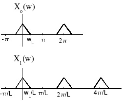
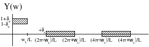

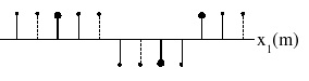


Figure 5.16.
So we need only control the filter response in the stopbands over the frequency regions with
nonzero energy. (Figure 5.17)
Figure 5.17.
The extra "don't care" bands allow a given set of specifications to be satisfied with a shorter-
length filter.
Direct polyphase filter design
Note that in an integer-factor interpolator, each set of output samples x 1( Ln+ p) ,
p={0, 1, …, L−1} , is created by a different polyphase filter gp( n) , which has no interaction with the other polyphase filters except in that they each interpolate the same signal. We can thus treat
the design of each polyphase filter independently, as an -length filter design problem.
Figure 5.18.
Each gp( n) produces samples
, where
is not an integer. That is, gp( n) is to
produce an output signal (at a T 0 rate) that is x 0( n) time-advanced by a non-integer advance .
The desired response of this polyphase filter is thus
for | ω|≤ π , an all-pass filter with a


linear, non-integer, phase. Each polyphase filter can be designed independently to approximate
this response according to any of the design criteria developed so far.
What should the polyphase filter for p=0 be?
A delta function: h 0( n)= δ( n′)
Example 5.2. Least-squares Polyphase Filter Design
Deterministic x(n): Minimize
Given x( n)= x( n)* h( n) and xd( n)= x( n)* hd( n) .
Using Parseval's theorem, this becomes
()
This is simply weighted least squares design, with (| X( ω)|)2 as the weighting function.
stochastic X(ω):
()
Sxx( ω) is the power spectral density of x. Sxx( ω)=DTFT[ rxx( k)]
Again, a
weighted least squares filter design problem.
Is it feasible to use IIR polyphase filters?
The recursive feedback of previous outputs means that portions of each IIR polyphase filter
must be computed for every input sample; this usually makes IIR filters more expensive than
FIR implementations.
5.5. Multistage Multirate Systems*

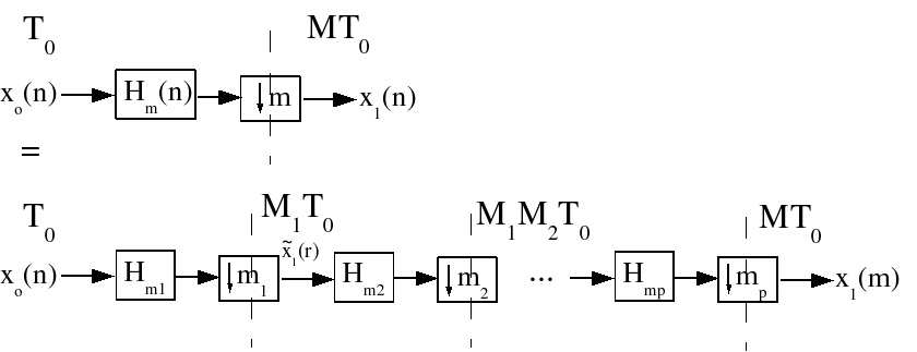


Multistage multirate systems are often more efficient. Suppose one wishes to decimate a signal by
an integer factor M, where M is a composite integer
. A decimator can be
implemented in a multistage fashion by first decimating by a factor M 1 , then decimating this
signal by a factor M 2 , etc. (Figure 5.19)
Figure 5.19. Multistage decimator
Multistage implementations are of significant practical interest only if they offer significant
computational savings. In fact, they often do!
The computational cost of a single-stage interpolator is:
The computational cost of a
multistage interpolator is:
The first term is the most significant, since the
rate is highest. Since ( Ni ∝ Mi) for a lowpass filter, it is not immediately clear that a multistage
system should require less computation. However, the multistage structure relaxes the
requirements on the filters, which reduces their length and makes the overall computation less.
Filter design for Multi-stage Structures
Ostensibly, the first-stage filter must be a lowpass filter with a cutoff at
, to prevent aliasing
after the downsampler. However, note that aliasing outside the final overall passband
is of
no concern, since it will be removed by later stages. We only need prevent aliasing into the band
; thus we need only specify the passband over the interval
, and the stopband over the
intervals
, for k∈{1, …, M−1} . (Figure 5.20)
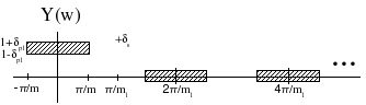


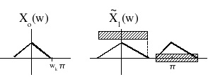
Figure 5.20.
Of course, we don't want gain in the transition bands, since this would need to be suppressed later,
but otherwise we don't care about the response in those regions. Since the transition bands are so
large, the required filter turns out to be quite short. The final stage has no "don't care" regions;
however, it is operating at a low rate, so it is relatively unimportant if the final filter turns out to
be rather long!
L-infinity Tolerances on the Pass and Stopbands
The overall response is a cascade of multiple filters, so the worst-case overall passband deviation,
assuming all the peaks just happen to line up, is
So one could
choose all filters to have equal specifications and require for each-stage filter. For ( δp ≪ 1) ,
ov
Alternatively, one can design later stages (at lower
computation rates) to compensate for the passband ripple in earlier stages to achieve exceptionally
accurate passband response.
δs remains essentially unchanged, since the worst-case scenario is for the error to alias into the
passband and undergo no further suppression in subsequent stages.
Interpolation
Interpolation is the flow-graph reversal of the multi-stage decimator. The first stage has a cutoff
at (Figure 5.21):
Figure 5.21.
However, all subsequent stages have large bands without signal energy, due to the earlier stages
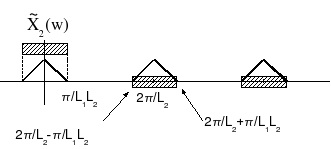

Figure 5.22.
The order of the filters is reversed, but otherwise the filters are identical to the decimator filters.
Efficient Narrowband Lowpass Filtering
A very narrow lowpass filter requires a very long FIR filter to achieve reasonable resolution in the
frequency response. However, were the input sampled at a lower rate, the cutoff frequency would
be correspondingly higher, and the filter could be shorter!
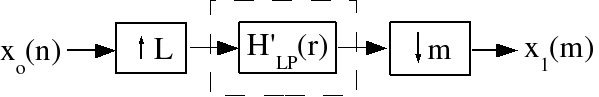
The transition band is also broader, which helps as well. Thus, Figure 5.23 can be implemented as
Figure 5.23.
Figure 5.24.
and in practice the inner lowpass filter can be coupled to the decimator or interpolator filters. If
the decimator and interpolator are implemented as multistage structures, the overall algorithm can
be dramatically more efficient than direct implementation!
5.6. DFT-Based Filterbanks*
One common application of multirate processing arises in multirate, multi-channel filter banks