| z|>| γ|
γn sin( αn) u[ n]
| z|>| γ|
Understanding Pole/Zero Plots on the Z-Plane*


Introduction to Poles and Zeros of the Z-Transform
It is quite difficult to qualitatively analyze the Laplace transform and Z-transform, since mappings of their magnitude and phase or real part and imaginary part result in multiple
mappings of 2-dimensional surfaces in 3-dimensional space. For this reason, it is very common to
examine a plot of a transfer function's poles and zeros to try to gain a qualitative idea of what a system does.
Once the Z-transform of a system has been determined, one can use the information contained in
function's polynomials to graphically represent the function and easily observe many defining
characteristics. The Z-transform will have the below structure, based on Rational Functions: ()
The two polynomials, P( z) and Q( z), allow us to find the poles and zeros of the Z-Transform.
Definition: zeros
1. The value(s) for z where
.
2. The complex frequencies that make the overall gain of the filter transfer function zero.
Definition: poles
1. The value(s) for z where
.
2. The complex frequencies that make the overall gain of the filter transfer function infinite.
Example 1.16.
Below is a simple transfer function with the poles and zeros shown below it.
The zeros are: {–1}
The poles are:
The Z-Plane
Once the poles and zeros have been found for a given Z-Transform, they can be plotted onto the Z-
Plane. The Z-plane is a complex plane with an imaginary and real axis referring to the complex-
valued variable z. The position on the complex plane is given by rⅇⅈθ and the angle from the
positive, real axis around the plane is denoted by θ. When mapping poles and zeros onto the plane,
poles are denoted by an "x" and zeros by an "o". The below figure shows the Z-Plane, and
examples of plotting zeros and poles onto the plane can be found in the following section.
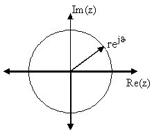


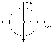


Figure 1.48. Z-Plane
Examples of Pole/Zero Plots
This section lists several examples of finding the poles and zeros of a transfer function and then
plotting them onto the Z-Plane.
Example 1.17. Simple Pole/Zero Plot
The zeros are: {0}
The poles are:
Figure 1.49. Pole/Zero Plot
Using the zeros and poles found from the transfer function, the one zero is mapped to zero and the two poles are placed at and
Example 1.18. Complex Pole/Zero Plot
The zeros are: { ⅈ, – ⅈ}

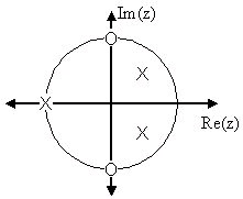


The poles are:
Figure 1.50. Pole/Zero Plot
Using the zeros and poles found from the transfer function, the zeros are mapped to ± ⅈ, and the poles are placed at –1,
and
Example 1.19. Pole-Zero Cancellation
An easy mistake to make with regards to poles and zeros is to think that a function like
is the same as s+3 . In theory they are equivalent, as the pole and zero at s=1 cancel
each other out in what is known as pole-zero cancellation. However, think about what may
happen if this were a transfer function of a system that was created with physical circuits. In
this case, it is very unlikely that the pole and zero would remain in exactly the same place. A
minor temperature change, for instance, could cause one of them to move just slightly. If this
were to occur a tremendous amount of volatility is created in that area, since there is a change
from infinity at the pole to zero at the zero in a very small range of signals. This is generally a
very bad way to try to eliminate a pole. A much better way is to use control theory to move
the pole to a better place.
Repeated Poles and Zeros
It is possible to have more than one pole or zero at any given point. For instance, the discrete-
time transfer function H( z)= z 2 will have two zeros at the origin and the continuous-time
function
will have 25 poles at the origin.
MATLAB - If access to MATLAB is readily available, then you can use its functions to easily
create pole/zero plots. Below is a short program that plots the poles and zeros from the above
example onto the Z-Plane.
% Set up vector for zeros
z = [j ; -j];
% Set up vector for poles
p = [-1 ; .5+.5j ; .5-.5j];
figure(1);
zplane(z,p);
title('Pole/Zero Plot for Complex Pole/Zero Plot Example');
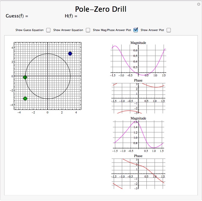
Interactive Demonstration of Poles and Zeros
Figure 1.51.
Interact (when online) with a Mathematica CDF demonstrating Pole/Zero Plots. To Download, right-click and save target as .cdf.
Applications for pole-zero plots
Stability and Control theory
Now that we have found and plotted the poles and zeros, we must ask what it is that this plot gives
us. Basically what we can gather from this is that the magnitude of the transfer function will be
larger when it is closer to the poles and smaller when it is closer to the zeros. This provides us

with a qualitative understanding of what the system does at various frequencies and is crucial to
the discussion of stability.
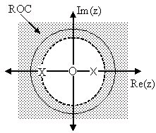
Pole/Zero Plots and the Region of Convergence
The region of convergence (ROC) for X( z) in the complex Z-plane can be determined from the
pole/zero plot. Although several regions of convergence may be possible, where each one
corresponds to a different impulse response, there are some choices that are more practical. A
ROC can be chosen to make the transfer function causal and/or stable depending on the pole/zero
plot.
Filter Properties from ROC
If the ROC extends outward from the outermost pole, then the system is causal.
If the ROC includes the unit circle, then the system is stable.
Below is a pole/zero plot with a possible ROC of the Z-transform in the Simple Pole/Zero Plot
discussed earlier. The shaded region indicates the ROC chosen for the filter. From this figure, we
can see that the filter will be both causal and stable since the above listed conditions are both met.
Example 1.20.
Figure 1.52. Region of Convergence for the Pole/Zero Plot
The shaded area represents the chosen ROC for the transfer function.
Frequency Response and Pole/Zero Plots
The reason it is helpful to understand and create these pole/zero plots is due to their ability to help
us easily design a filter. Based on the location of the poles and zeros, the magnitude response of
the filter can be quickly understood. Also, by starting with the pole/zero plot, one can design a
filter and obtain its transfer function very easily.
Glossary
Definition: difference equation
An equation that shows the relationship between consecutive values of a sequence and the
differences among them. They are often rearranged as a recursive formula so that a systems
output can be computed from the input signal and past outputs. Example .
simplemath mathml-miitalicsy[ mathml-miitalicsn]+7 mathml-miitalicsy[ mathml-miitalicsn−1]+2
Definition: poles
1. The value(s) for simplemath mathml-miitalicsz z where Qz= .
2. The complex frequencies that make the overall gain of the filter transfer function infinite.
Definition: zeros
1. The value(s) for simplemath mathml-miitalicsz z where Pz= .
2. The complex frequencies that make the overall gain of the filter transfer function zero.
Solutions
Chapter 2. Digital Filter Design
2.1. Overview of Digital Filter Design*
Advantages of FIR filters
1. Straight forward conceptually and simple to implement
2. Can be implemented with fast convolution
3. Always stable
4. Relatively insensitive to quantization
5. Can have linear phase (same time delay of all frequencies)
Advantages of IIR filters
1. Better for approximating analog systems
2. For a given magnitude response specification, IIR filters often require much less computation
than an equivalent FIR, particularly for narrow transition bands
Both FIR and IIR filters are very important in applications.
Generic Filter Design Procedure
1. Choose a desired response, based on application requirements
2. Choose a filter class
3. Choose a quality measure
4. Solve for the filter in class 2 optimizing criterion in 3
Perspective on FIR filtering
Most of the time, people do L∞ optimal design, using the Parks-McClellan algorithm. This is probably the second most important technique in "classical" signal processing (after the Cooley-
Tukey (radix-2) FFT).
Most of the time, FIR filters are designed to have linear phase. The most important advantage of
FIR filters over IIR filters is that they can have exactly linear phase. There are advanced design
techniques for minimum-phase filters, constrained L 2 optimal designs, etc. (see chapter 8 of text).
However, if only the magnitude of the response is important, IIR filers usually require much
fewer operations and are typically used, so the bulk of FIR filter design work has concentrated on
linear phase designs.
2.2. FIR Filter Design
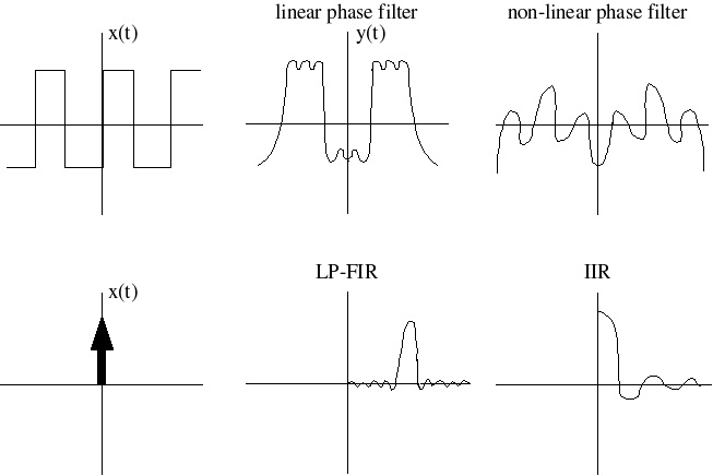
Linear Phase Filters*
In general, for – π≤ ω≤ π H( ω)=| H( ω)| ⅇ–( ⅈθ( ω)) Strictly speaking, we say H( ω) is linear phase if H( ω)=| H( ω)| ⅇ–( ⅈωK) ⅇ–( ⅈθ 0) Why is this important? A linear phase response gives the same time delay for ALL frequencies! (Remember the shift theorem.) This is very desirable in many
applications, particularly when the appearance of the time-domain waveform is of interest, such as
in an oscilloscope. (see Figure 2.1)


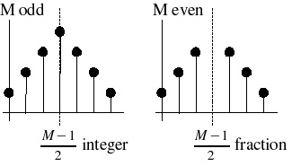
Figure 2.1.
Restrictions on h(n) to get linear phase
()
For linear phase, we require the right side of Equation to be ⅇ–( ⅈθ 0)(real,positive function of ω) .
For θ 0=0 , we thus require
h(0)+ h( M−1)=real number h(0)− h( M−1)=pure imaginary number h(1)+ h( M−2)=pure real number h(1)− h( M−2)=pure imaginary number ⋮ Thus h( k)= h*( M−1− k) is a necessary condition for the right side of Equation to be real valued, for θ 0=0 .
For
, or ⅇ–( ⅈθ 0)=– ⅈ , we require
h(0)+ h( M−1)=pure imaginary h(0)− h( M−1)=pure real number ⋮ ⇒ h( k)=–( h*( M−1− k)) Usually, one is interested in filters with real-valued coefficients, or see Figure 2.2 and Figure 2.3.
Figure 2.2.
θ 0=0 (Symmetric Filters). h( k)= h( M−1− k).
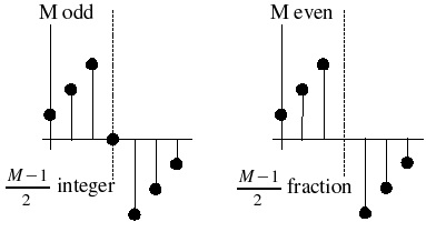


Figure 2.3.
(Anti-Symmetric Filters). h( k)=–( h( M−1− k)).
Filter design techniques are usually slightly different for each of these four different filter types.
We will study the most common case, symmetric-odd length, in detail, and often leave the others
for homework or tests or for when one encounters them in practice. Even-symmetric filters are
often used; the anti-symmetric filters are rarely used in practice, except for special classes of
filters, like differentiators or Hilbert transformers, in which the desired response is anti-
symmetric.
So far, we have satisfied the condition that
where A( ω) is real-valued.
However, we have not assured that A( ω) is non-negative. In general, this makes the design
techniques much more difficult, so most FIR filter design methods actually design filters with
Generalized Linear Phase:
, where A( ω) is real-valued, but possible negative.
A( ω) is called the amplitude of the frequency response.
Excuse
A( ω)
Example 2.1.
Lowpass Filter
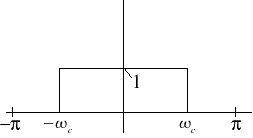
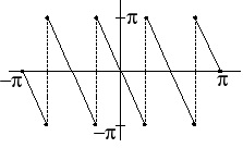

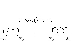
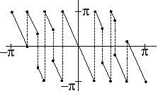

Figure 2.4. Desired |H(ω)|
Figure 2.5. Desired ∠H(ω)
The slope of each line is
.
Figure 2.6. Actual |H(ω)|
A( ω) goes negative.
Figure 2.7. Actual ∠H(ω)
2 π phase jumps due to periodicity of phase. π phase jumps due to sign change in A( ω) .
Time-delay introduces generalized linear phase.
For odd-length FIR filters, a linear-phase design procedure is equivalent to a zero-phase
design procedure followed by an
-sample delay of the impulse response. For even-
length filters, the delay is non-integer, and the linear phase must be incorporated directly
in the desired response!


Window Design Method*
The truncate-and-delay design procedure is the simplest and most obvious FIR design procedure.
Is it any Good?
Yes; in fact it's optimal! (in a certain sense)
L2 optimization criterion
find h[ n] , 0≤ n≤ M−1 , maximizing the energy difference between the desired response and the actual response: i.e., find
()
Since
this becomes
h[ n]
The best we can do is let
Thus h[ n]= hd[ n] w[ n] ,
is
optimal in a least-total-sqaured-error ( L 2 , or energy) sense!
Why, then, is this design often considered undersirable?
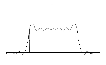
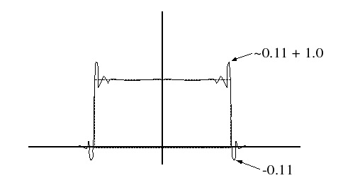

(b) A( ω) , large M
(a) A( ω) , small M
Figure 2.7.
For desired spectra with discontinuities, the least-square designs are poor in a minimax (worst-
case, or L∞ ) error sense.
Window Design Method
Apply a more gradual truncation to reduce "ringing" (Gibb's Phenomenon)
H( ω)= Hd( ω)* W( ω)
The window design procedure (except for the boxcar window) is ad-hoc and not optimal in any
usual sense. However, it is very simple, so it is sometimes used for "quick-and-dirty" designs of if
the error criterion is itself heurisitic.
Frequency Sampling Design Method for FIR filters*
Given a desired frequency response, the frequency sampling design method designs a filter with a
frequency response exactly equal to the desired response at a particular set of frequencies ωk .
(2.1)
Procedure
Desired Response must incluce linear phase shift (if linear phase is desired)


What is Hd( ω) for an ideal lowpass filter, cotoff at ωc ?
This set of linear equations can be written in matrix form
(2.2)
(2.3)
or
So
(2.4)
W N= M ωi≠ ωj+ 2πl i≠ j
Important Special Case
What if the frequencies are equally spaced between 0 and 2 π , i.e.
Then
so
or
Important Special Case #2
h[ n] symmetric, linear phase, and has real coefficients. Since h[ n]= h[ M−